
Whenever we run OLS regressions, there are a few basic assumptions that are made with regard to our data so that correct inferences and predictions can be made. To learn the basics of regression assumption, please refer to an introductory textbook on econometrics. The four regression assumptions that we will discuss in this article are as follows:
- Normality of residuals
- Heteroskedasticity
- Multicollinearity
- Autocorrelation
These four assumptions apply for any kind of dataset, regardless of it being a cross-sectional data, panel data, or time-series data.
To test the four regression assumptions, we will use Stata’s built-in automobile dataset.
sysuse auto, clear
Testing the Normality of Residuals as regression assumptions in Stata
Related Article: How To Check Normality of a Variable In Stata
The first regression assumption states that the residuals obtained after a regression must be normally distributed. Remember, it does not matter if our dependent or independent variables are normally distributed or not.
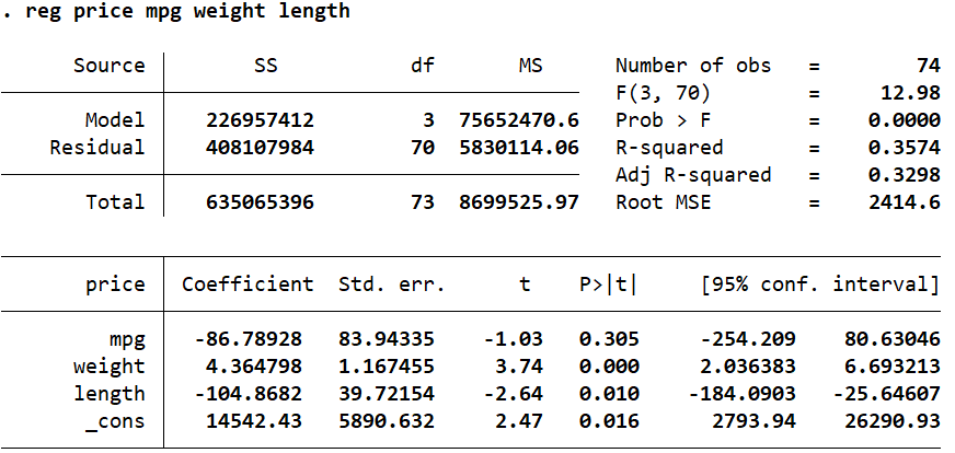
We can check the normality of residuals in Stata by first running the regression and then obtaining the residuals to be observed. Our dependent variable is ‘price’, and our independent variables/regressors are ‘mpg’, ‘weight’ and ‘length’.
reg price mpg weight length
The command predict can then be used after the regression to create a new variable with the regression residuals. The residuals from the following command will be stored in a variable called ‘error’. The option residual specifies that we need the residuals from the regression to be reported. Other statistics like the predicted values of the dependent variable, standard errors etc. can also be obtained using the predict – explore these possibilities using the command: help predict.
Essentially, this command tells Stata to get the predicted residuals from the regression that was run in a previous command, and store them in a new variable called ‘error’.
predict error, residual
We now have a new variable called ‘error’ which stores the residual value for each observation. In order to determine its distribution, let’s summarize it in detail.
summarize error, detail
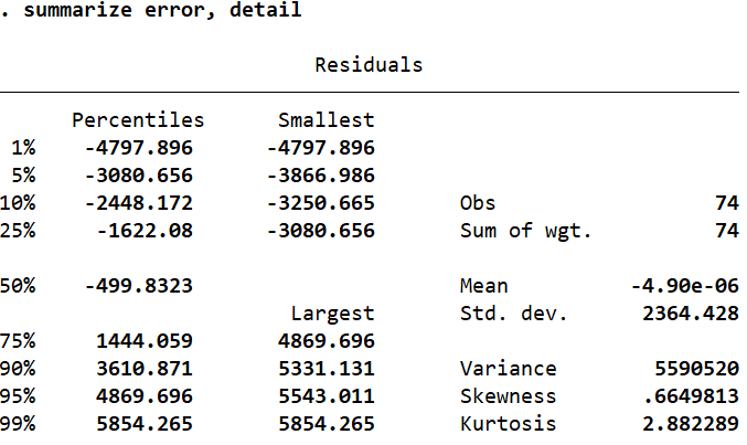
If the skewness value is close to zero, we can infer that a variable is neither positively nor negatively skewed. The skewness of ‘error’ is 0.66 which is sufficiently close to zero to suggest that the residuals are indeed normally distributed. Similarly, if the kurtosis value is 3, we can again conclude that a variable is normally distributed (here, kurtosis is very close to 3 with a value of 2.88).
In some statistical software packages, the kurtosis value is reported as a difference from 3. When interpreting these, the kurtosis value will be compared to zero to determine normality.
Skewness and kurtosis are simple summary statistics that are not accompanied by any statistical tests to indicate their significance.
The Skewness and Kurtosis Test for Normality in Stata
A test of significance of the skewness and kurtosis can be performed for the residual variable using the sktest command (the skewness and kurtosis tests for normality).
sktest error
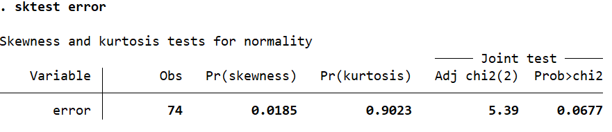
The null hypothesis of this test is that the data is normally distributed, satisfying regression assumption. A p-value (Prob>chi2) of less than 0.05 would indicate that the variable is not normally distributed. In this case, it is just above this value at 0.0677 which can allow us to infer that the variable is indeed normally distributed.
The Shapiro-Wilk Test for Normality in Stata
Let’s also run a Shapiro-Wilk test of normality using the swilk command. This gives us the following output.
swilk error
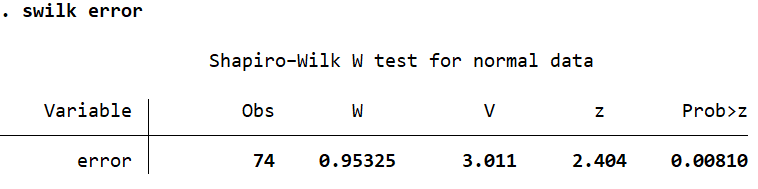
The p-value (Prob>z) in this case is 0.0081 which is well below 0.05. This test leads us to reject the null hypothesis of a normal distribution, and conclude that the residuals are not normally distributed. This is primarily because these tests have a bias to (i.e they are sensitive to) sample sizes. In large sample sizes, they tend to indicate significance even if there is a small deviation from normality.
The Jarque-Bera Test for Normality in Stata
There is another command, jb, that performs that Jarque-Bera normality test. You may have to install it before using it.
ssc install jb jb error
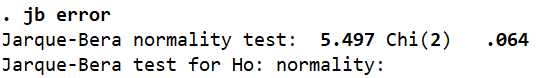
This test gives us a p-value of 0.064 whereby we fail to reject the null hypothesis of normality of residuals and conclude that ‘error’ is normally distributed.
Multiple Scatter Plots on One Graph in Stata
Related Article: Scatter plots in Stata
Generally speaking, if we wanted to get a visual representation of multiple variables as scatter plots, separate scatter plots for each of the variables would need to be produced. To get around this issue, we can generate the scatter plots of multiple variables using the graph matrix command.
graph matrix price mpg weight length
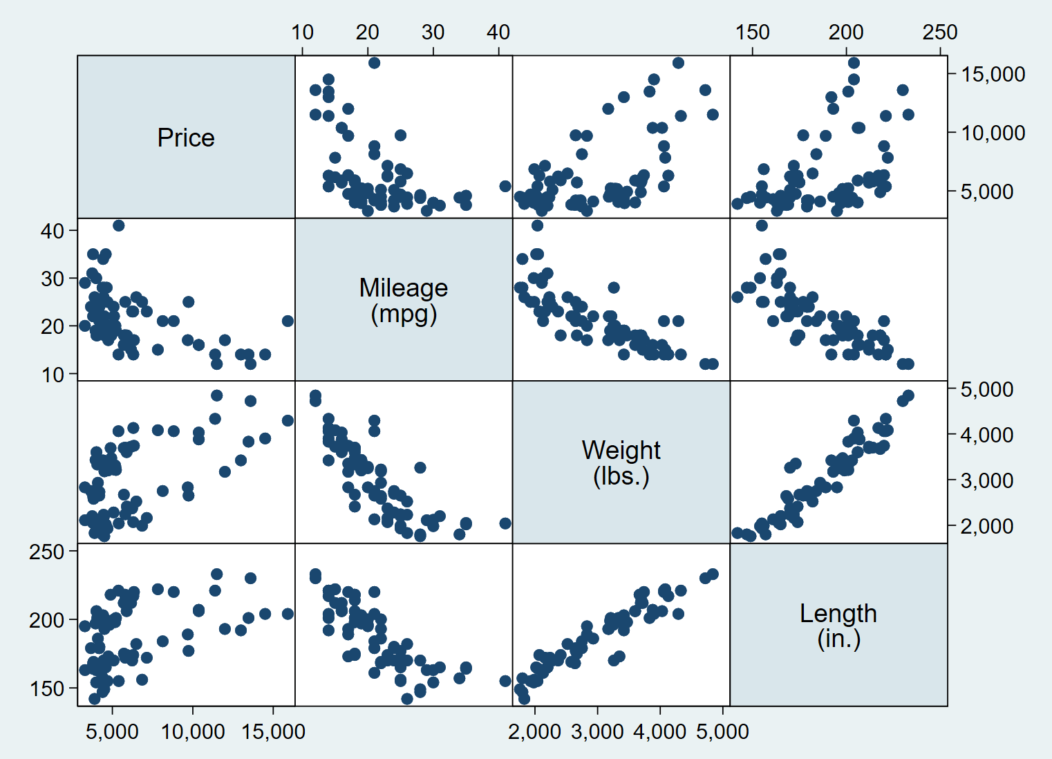
The multiple graphs generated by the command give us the two way scatterplots of all the combinations of the variables we specified.
The normality of a variable can also be visualised by plotting certain graphs in Stata.
The Standardised Normal Probability Plot
The pnorm command generates a standardised normal probability plot. The closer the plotted points are to the straight line, the more likely it is for the variable to be normally distributed. If the data points lie exactly on the straight line, the variable can be said to be perfectly normally distributed.
pnorm error
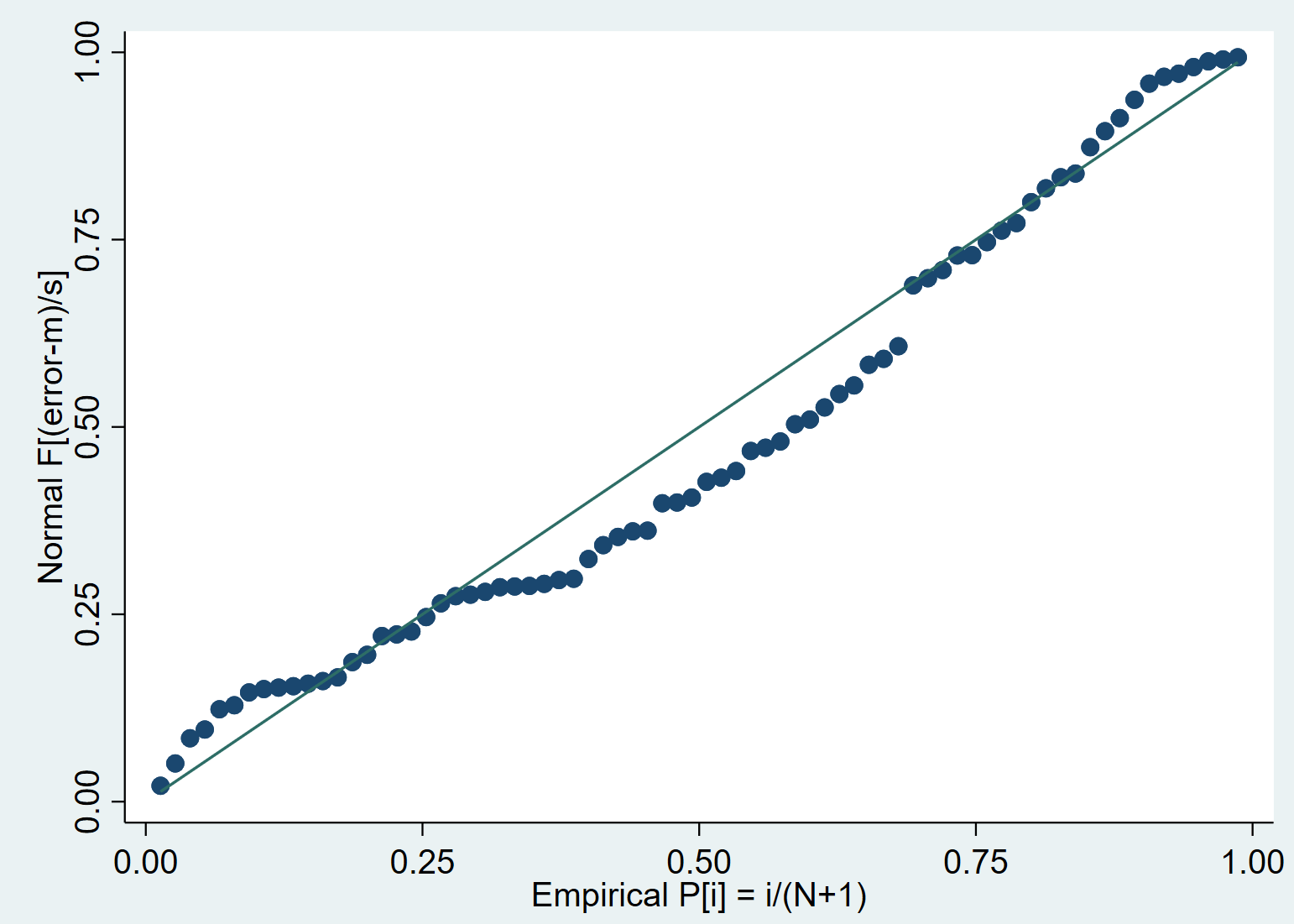
In this case, the data points are quite close to the straight line and help us visually conclude that ‘error’ is a normally distributed variable.
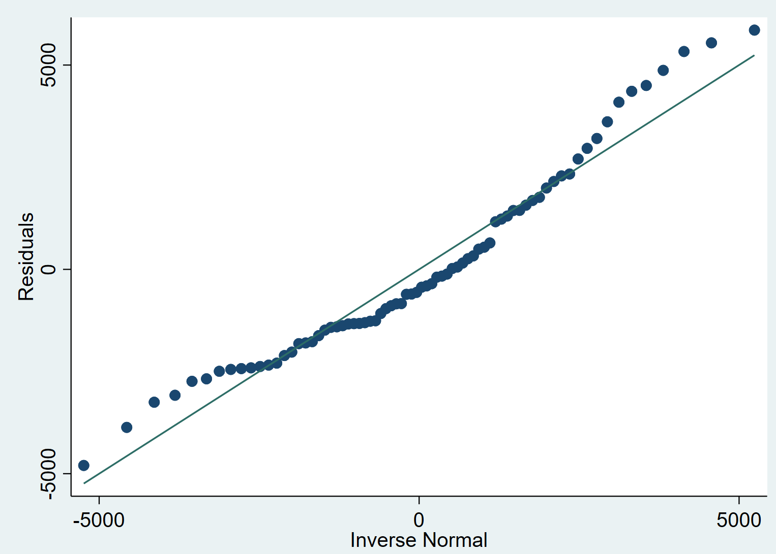
The Normal Quantile Plot to test regression Assumptions
A quantile plot helps us visualize normality in exactly the same manner. The command qnorm plots the quantiles of the variable specified against the quantiles of normal distribution.
qnorm error
What to do if The Normality Assumption is Violated?
Reporting Unbiased Standard Errors in a Regression
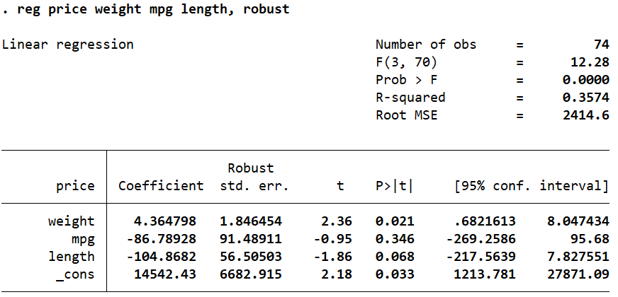
If the residuals from a simple OLS regression are not normally distributed, you should make inferences about the coefficients based on robust, corrected, unbiased standard errors. Unbiased standard errors in a regression can be reported by adding the option robust to a regression command.
reg price weight mpg length, robust
The vce Option to Correct Biased Standard Errors
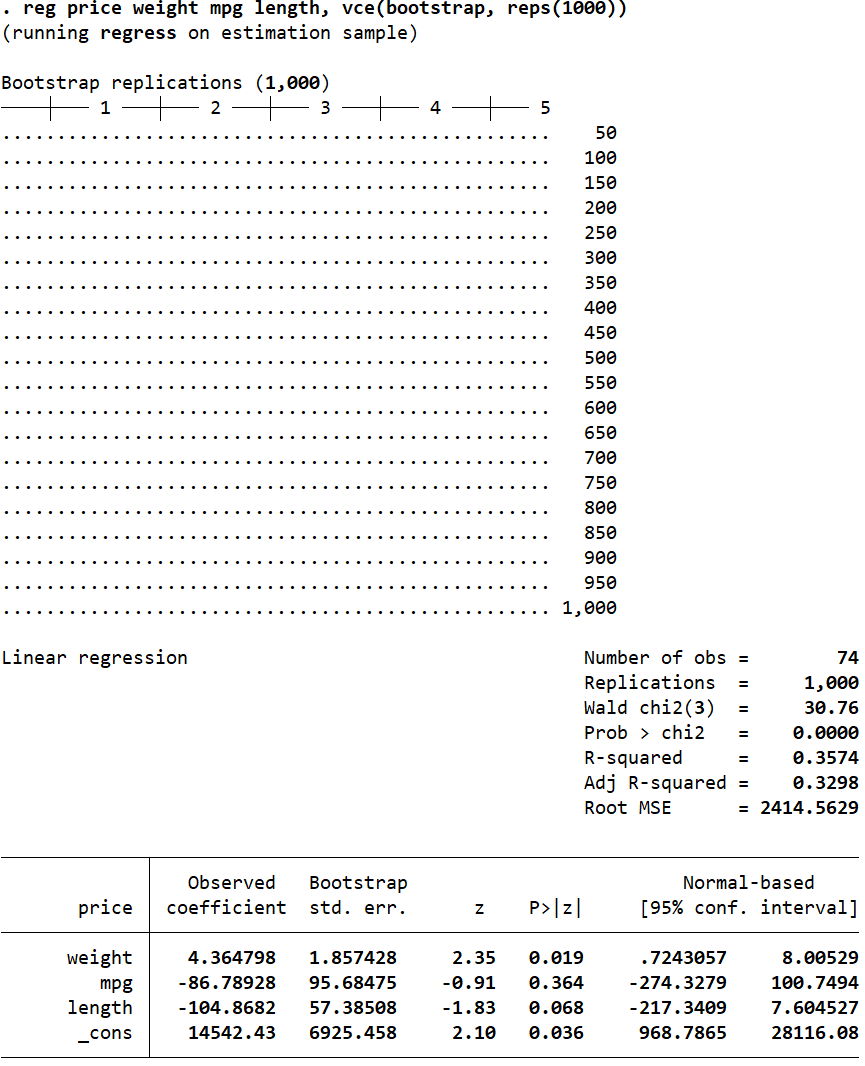
Another way of correcting biased standard errors is to have Stata draw multiple random samples from our data, run the regression for all of these samples, and report an average of all the estimates in the output.
The vce(bootstrap, reps(number_of_repetitions) option can help obtain bias-corrected standard errors and confidence intervals.
reg price weight mpg length, vce(bootstrap, reps(1000))
Related Article: Estimate Multiple Regression In Stata
Testing the Heteroskedasticity as regression assumptions in Stata
Heteroskedasticity is a violation of the homoskedasticity (constant variance) assumption. This means that variability in our outcome variable changes as the independent variable increases. For example, in a regression of savings on earnings, we may find that individuals with lower income save very little, but individuals with higher incomes may save too much or too little. In other words, the residuals do not have a constant variance. Heteroskedasticity leads to biased standard errors and incorrect inferences.
Visualizing Heteroskedasticity in Stata
Let’s visualize heteroskedasticity. For the regression that we ran above, the residuals and the predicted outcome variable can be plotted on a graph.
reg price mpg weight length
The following two commands will generate a variable ‘resid’ to store the regression residuals, and another variable called ‘yhat’ to store the predicted values of the outcome variable.
predict resid, residuals predict yhat, xb
We can now plot these variables using the rvfplot command (rvfplot is short for ‘residuals vs fitted plot’). The option yline(0) will be used to draw a line at 0 which can be used to observe the variance of the residuals.
rvfplot, ytitle(resid) yline(0) xtitle(yhat)
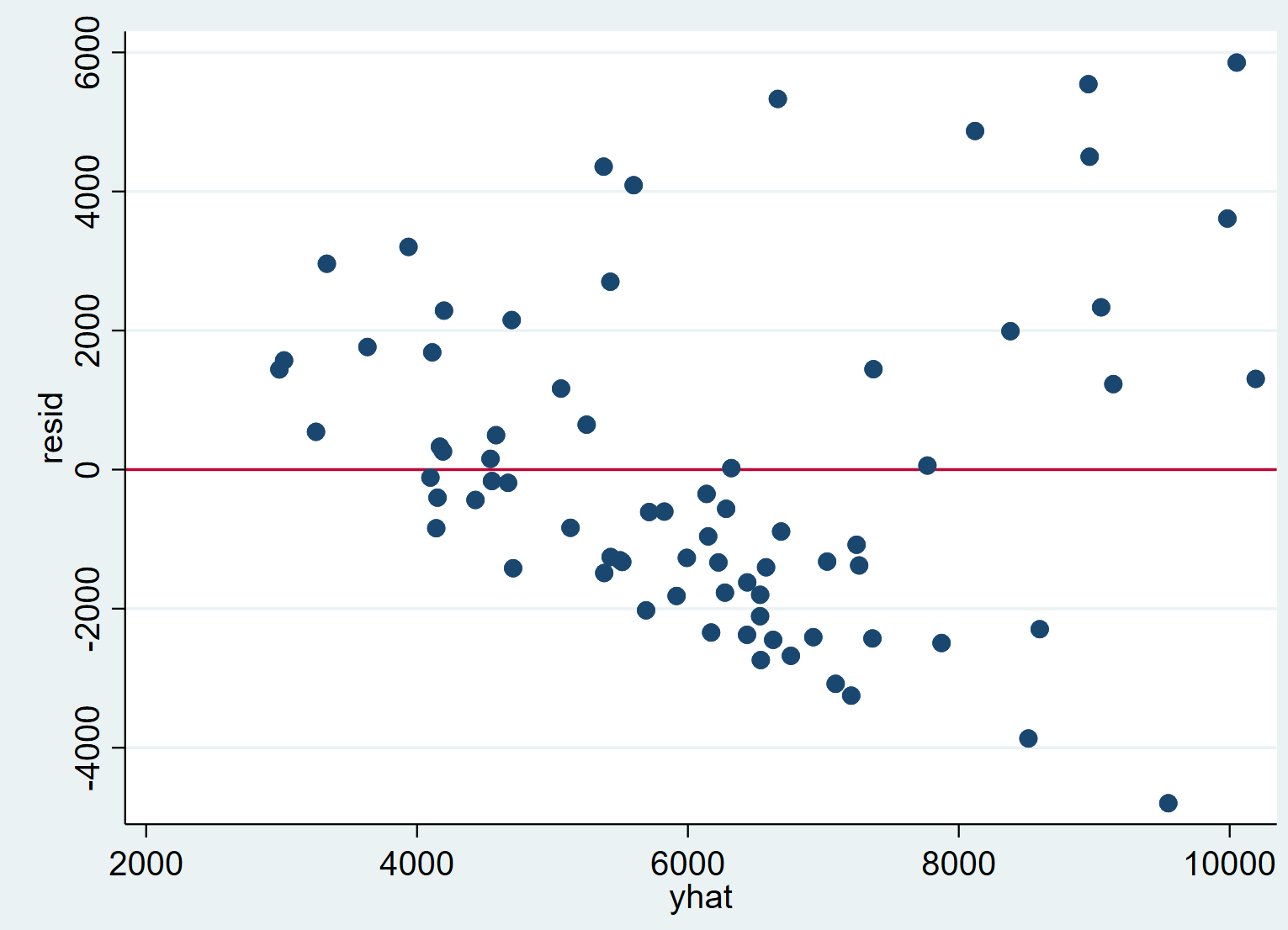
It is evident that with higher fitted values, residuals of the regression tend to adopt a greater variance. The cone shape of the scatter plot confirms that heteroskedasticity is a problem in this regression.
Heteroskedasticity can be (more reliably) confirmed using statistical tests as well.
The Cameron-Trivedi Decomposition of the IM-Test
The Cameron-Trivedi decomposition of the IM-test can be performed after a regression using the estat imtest command which includes a test for heteroskedasticity as well.
reg price mpg weight length estat imtest
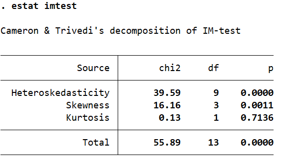
The null hypothesis for this test assumes homoskedasticity. If the p-value in the far-right column is less than 0.05, the assumption is violated (the null is rejected) and heteroskedasticity is considered to be present.
The Breusch-Pagan Test for Heteroskedasticity
The Bresuch-Pagan test for heteroskedasticity can be performed using the estat hettest command.
estat hettest
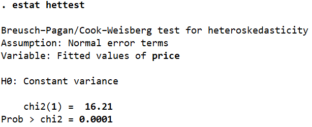
As indicated, the test assumes that the error terms are normal or homoskedastic. If the p-value (Prob > chi2) is less than 0.05, we reject this assumption of the null hypothesis and conclude that our residuals/errors are heteroskedastic. In this case, the p-value is 0.0001, well below 0.05.
Testing the Multicollinearity as regression assumptions in Stata
Multicollinearity means that the independent variables in a regression are correlated. One of the regression assumptions is that multicollinearity is not present. Multicollinearity can lead to large and inflated standard errors, which in turn will lead us to (often wrongly) infer that a coefficient is statistically insignificant when in reality it is significant.
The Correlation Matrix
Related Article: Correlation Analysis in Stata (Pearson, Spearman, Listwise, Casewise, Pairwise)
The correlation between variables can be checked using the corr command.
corr price mpg weight length
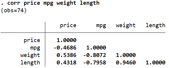
In this case,we can see that ‘mpg’ is highly (negatively) correlated with ‘weight’ and ‘length’, and the latter two are also strongly (positively) correlated with each other (0.9460).
However, the appropriate way to determine multicollinearity in Stata is by reporting the variance inflation factor for each independent variable after a regression.
The Variance Inflation Factor
reg price mpg weight length vif
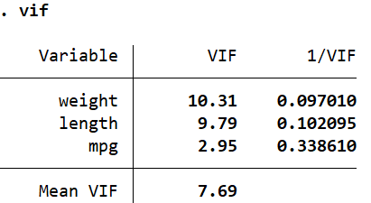
Alternatively, you can also run estat vif to report exactly the same table.
The value in the first column ‘VIF’ should be less than 10 if we are to rule out multicollinearity. If it is greater than 10, the problem of multicollinearity exists. Sometimes, the mean of all the VIF values (Mean VIF which is 7.69 here) is also compared against 1. If this mean value is greater than 1, there is evidence of multicollinearity.
The second column, ‘1/VIF’ reports the tolerance levels. If a tolerance level is less than 0.1, multicollinearity is suspected. The tolerance level can also be interpreted by subtracting it from 1 and then multiplying the resulting value by 100 to obtain a percentage. For example, (1 – 0.097) * 100 = 90.3%. This means that 90.3% of the variation explained by ‘weight’ is also explained by other variables. Only 9.7% of the explained variation is unique to ‘weight’.
This makes sense, since it is very likely that a car with a higher ‘weight’ also has more ‘length’. The problematic variable in case of multicollinearity is often dropped because the information it offers is also provided by the other variable that it is correlated with.
Let’s drop ‘weight’ and reobtain the VIF values.
reg price mpg length estat vif
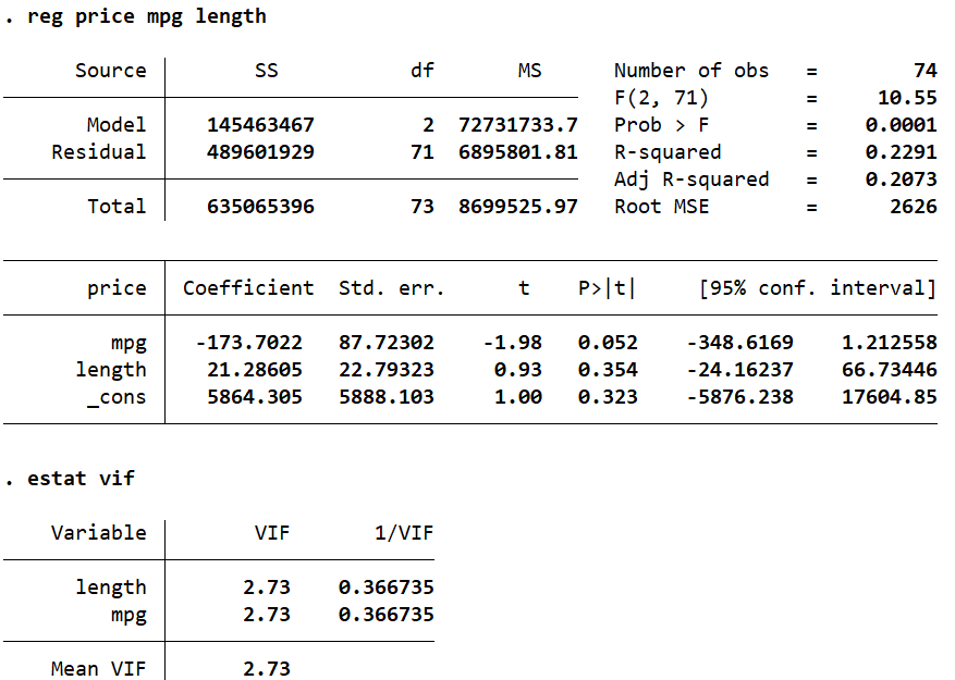
Dropping ‘weight’ from our regression dramatically reduces the VIF values for the other two variables, which in turn helps mitigate the problem of multicollinearity as well, satisfying regression assumptions.
Autocorrelation
The fourth regression assumption is no autocorrelation in data. The problem of autocorrelation occurs when residuals of a data set are correlated with each other. This violates the regression assumption that residuals are independent of each other and don’t exhibit any systematic patterns over time in time series data. However, when errors are correlated, it leads to biased regression results. It is therefore important to check for autocorrelation in data, and if problem of autocorrelation exists, it should be corrected accordingly.
Checking for autocorrelation in Stata
Autocorrelation is the issue of time series data, so we need to set data to time series. To instruct Stata to change data to time series, we need to generate a new variable by using following command
gen trend = _n
To further instruct the Stata about changing data setting to time series, we use the command as follows
tsset trend
Once the data has been set to time series, we move forward to checking for autocorrelation in our data. However, first we run a regression by using following command
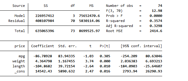
reg price mpg weight length
The following regression results are generated
Now, to test for autocorrelation, there exists different tests. These tests include Durbin Watson test and Breusch–Godfrey LM test. We will go through them individually.
To run Durbin Watson test in stata, use the following command
dwstat
This will generate following results of Durbin Watson test.
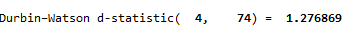
The Durbin Watson test values range from 0 to 4, where 2 means no auto correlation, values less than 2 mean positive autocorrelation and values above than 2 mean negative correlation. In this case, as we can see, the Durbin Watson test value is 1.2768 which is lower than 2, thus indicating that positive autocorrelation exists in data.
The next test for identification of autocorrelation in data is Breusch–Godfrey LM test. This test has advantage over Durbin Watson test, which it allows you to test for autocorrelation over more than 1 lag. To run the Breusch–Godfrey LM test, use the following command
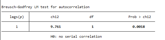
estat bgodfrey
This command generates the following results. Interpreting results, we can see that the associated p-value is 0.0018, which is less than the commonly used significance level of 0.05. Therefore, there is strong evidence to reject the null hypothesis of no autocorrelation. The autocorrelation, thus exists in data.
Correcting for Autocorrelation
The most commonly used method for correcting the issue of autocorrelation is by using the prais command in Stata. The prais command in Stata is used to estimate a random-effects model with spatial error structure, also known as the Prais-Winsten transformation This transformation is often used when the data have both serial correlation (autocorrelation) and spatial correlation. To correct for autocorrelation, use the following command
prais price mpg weight length, corc
The prais is used in place of regress function in Stata, and this will correct for the issue of autocorrelation by transformation. The results generated by the above command is are as following
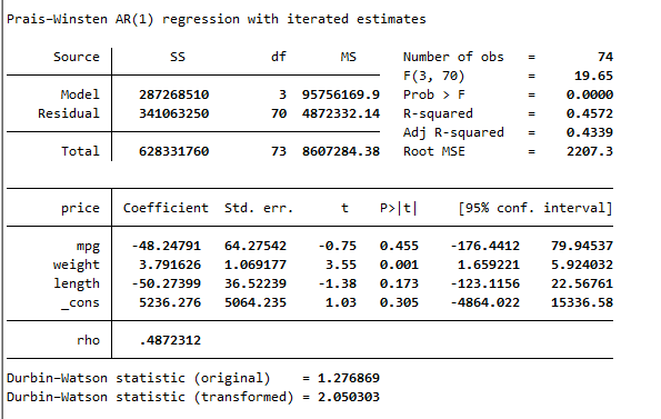
The results of Durbin Watson test are given below, which indicates that value of Durbin Watson test after transformation is 2.05, verifying that issue of autocorrelation has been resolved using the in-built function in Stata.