
In this blog, we are going to introduce you to one of the most famous models in the asset pricing model. Back then in 1993 two researchers (Fama and French) in finance created a model, which proved that three risk factors (market risk premium, size, and value) can statistically and significantly explain the fluctuations of stock returns in the USA. After several years in 2015, they decided to add two other risk factors to the well-known Fama and French three-factor model. These two additional factors were investment and profitability. This five-factor model had a high explanatory power like the previous model in 1993, with a little difference in that the value factor appeared to be redundant.
The main goal of this blog is to show how we can replicate the factors and construct the Fama and French portfolios in the three-factor model, and we broke down the blog into the following points:
- Capital Asset Pricing Model (CAPM) versus Fama and French Model (FFM)
- Portfolio Construction
- Univariate Portfolio
- Bivariate Independent Sort
- Bivariate Dependent Sort
- SMB (size factor) and HML (value factor) Construction
CAPM VS FFM
Let’s begin with the first part, which compares the CAPM and FFM with each other. In 1964 William Sharpe introduced a model, which shows that the market risk premium is the only factor that can explain the variations in the stock returns. The model which he created is illustrated in the equation (1).

Where:
E(Ri) is the expected return of a stock
Rf is the risk-free rate
bi is the systematic risk or the coefficient of the market risk premium
Rm – Rf is the market risk premium
As we can see equation (1) has only one factor and because of that it is known as a single-factor model. If we add at least two additional factors to the model it will be named a multi-factor model like the model which was proposed by Fama and French in 1993. This model is indicated in equation (2) below:

Where:
SMB stands for small minus big which is the size factor
HML stands for high minus low which is the value factor
Univariate VS Bivariate
Now it is time to construct the portfolios for our further analysis. As mentioned earlier, we have two portfolio construction methods: 1- Univariate and 2- Bivariate. But what are the differences between these two groups?
Univariate Portfolio Construction
Whenever we construct a portfolio only based on one factor we call it a univariate portfolio, but if the portfolio is constructed based on at least two factors, then we have a bivariate portfolio. Example 1: Let’s explain them with the help of two examples to ease the understanding of the concept.
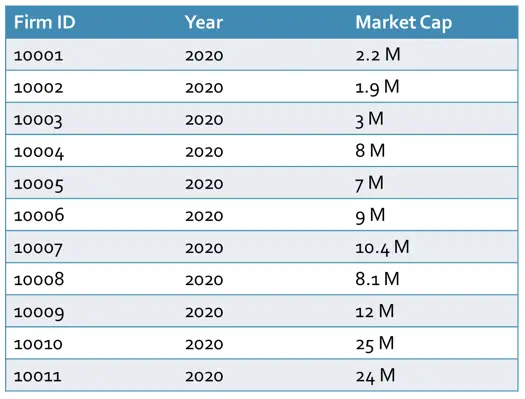
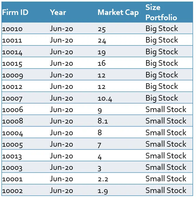
Imagine that we have market capitalizations of different companies in the year 2020 according to the figure above. We want to categorize the firms as small and big. First, we need to calculate the median which is 8.05 in this case. Then we put each firm or stock in their appropriate group according to the figure below.
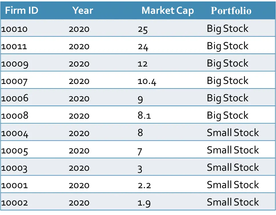
Note: In our example, the stock prices have monthly intervals, and the portfolios are reconstructed once a year, which is very common in asset pricing studies. But you may also use other intervals.
After sorting our firms based on the size, we need their stock returns to calculate the return of each portfolio. We have added the stock returns in the last column of the following table.
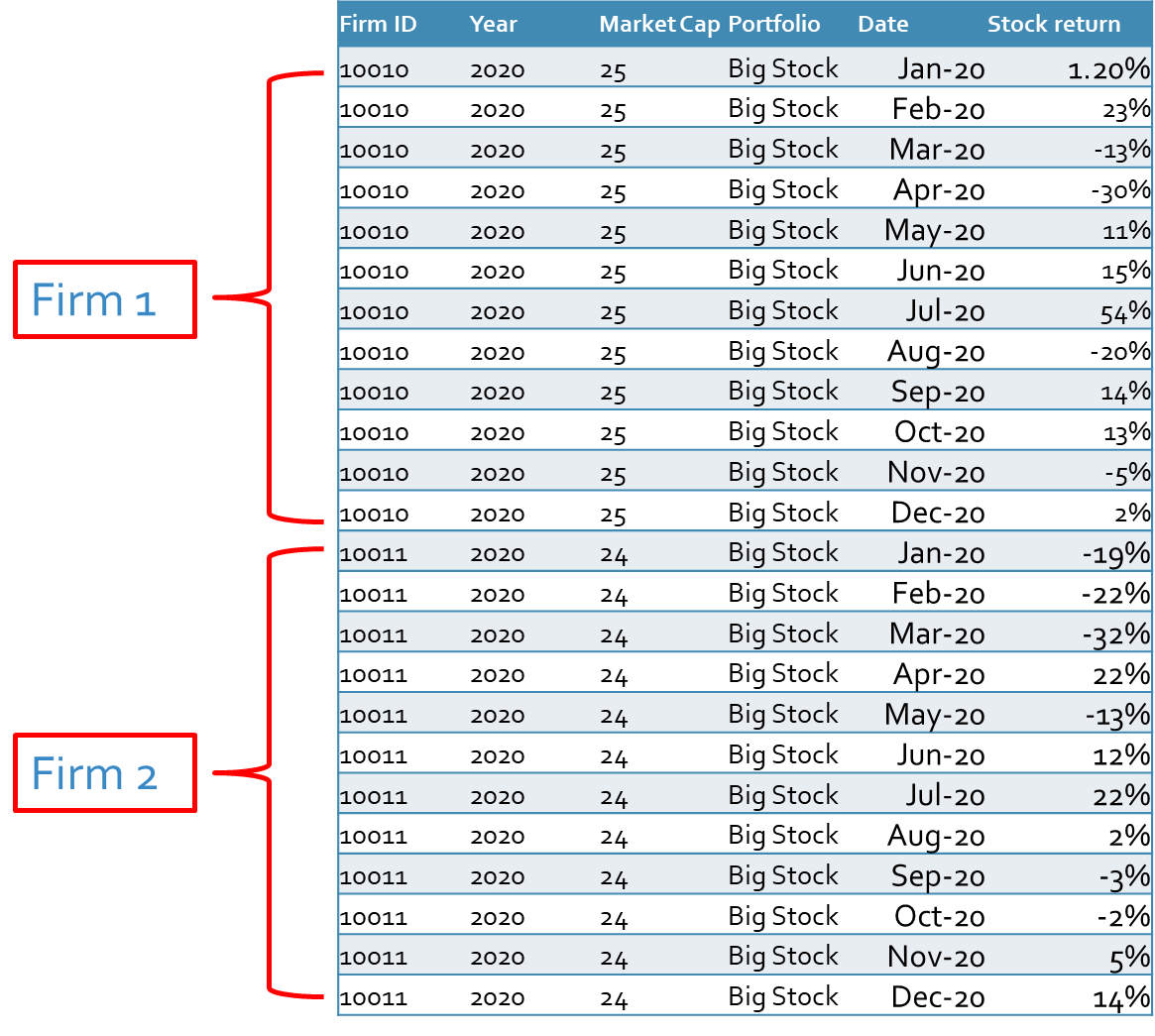
As you can see, we have several stock returns (firm 1, firm 2, firm 3, …) for each portfolio in each month. To calculate the portfolio stock returns we need to make the average of all returns for each portfolio in each month. This could be either value-weighted or equal-weighted average return. In the examples of this blog, we used the equal-weighted method, however, we recommend you use the value-weighted method, which gives you more accurate results because of the diversification effect.
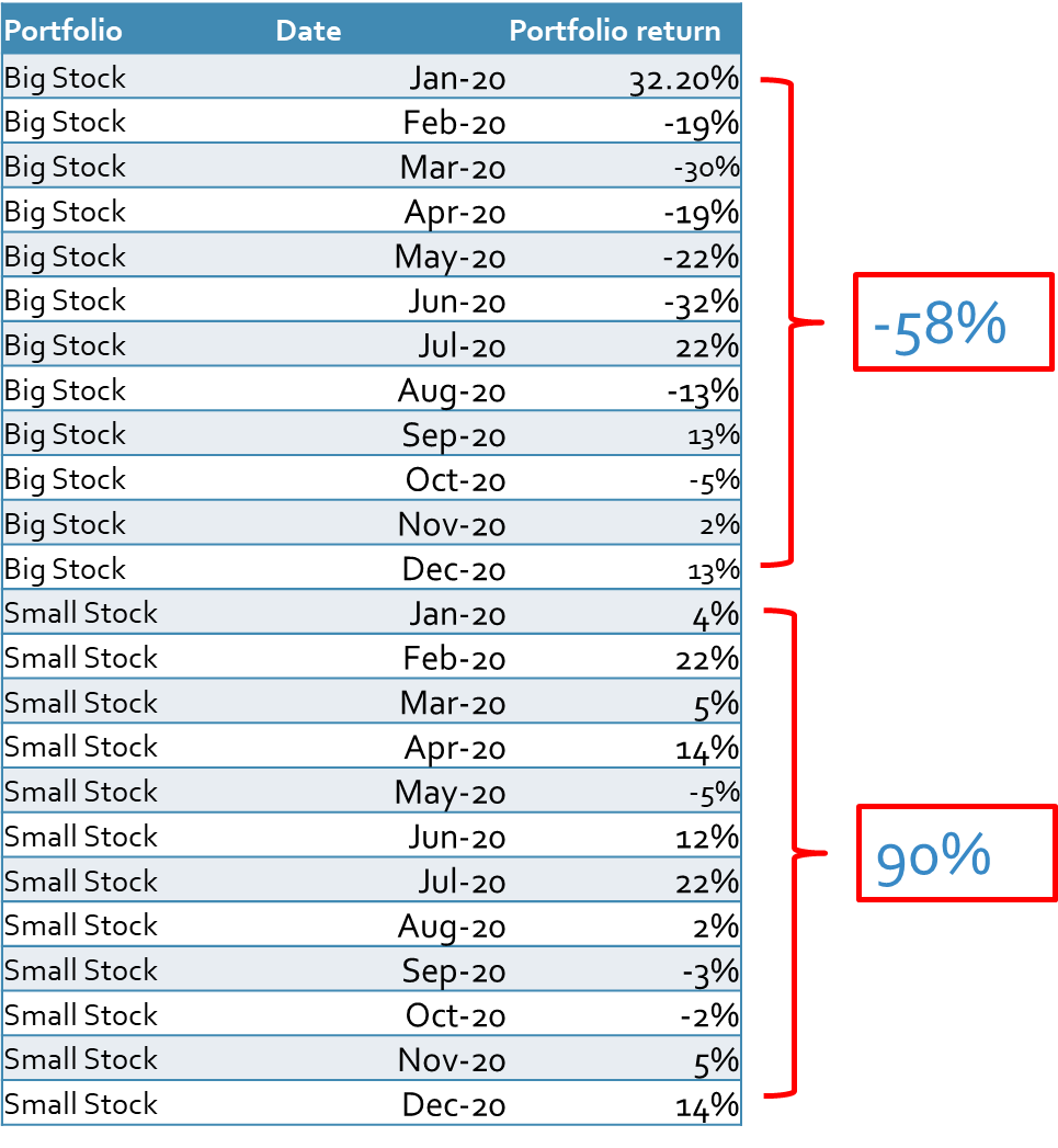
One interesting point is that small stocks have on average higher returns than big stocks, which was already proved by Fama and Frech and other studies. If you take a simple average of all big stocks, then we have -58% and 90% for small stocks. One reason could be the higher volatilities of small stocks which are subject to that small stocks record higher prices in comparison to big stocks.
Bivariate Portfolio Construction
The second type of portfolio construction is bivariate which itself is divided into two groups: 1- Independent sort and 2- Dependent sort.
Independent Sort
Independent sort is exactly what we explained earlier. It means we calculate the breakpoints of each factor regardless of the breakpoints of the other factor, or it does not make any difference whether to start to sort the firms based on the first factor and then the second factor or vice versa. Please follow the example below to make sure that you understand this method completely.
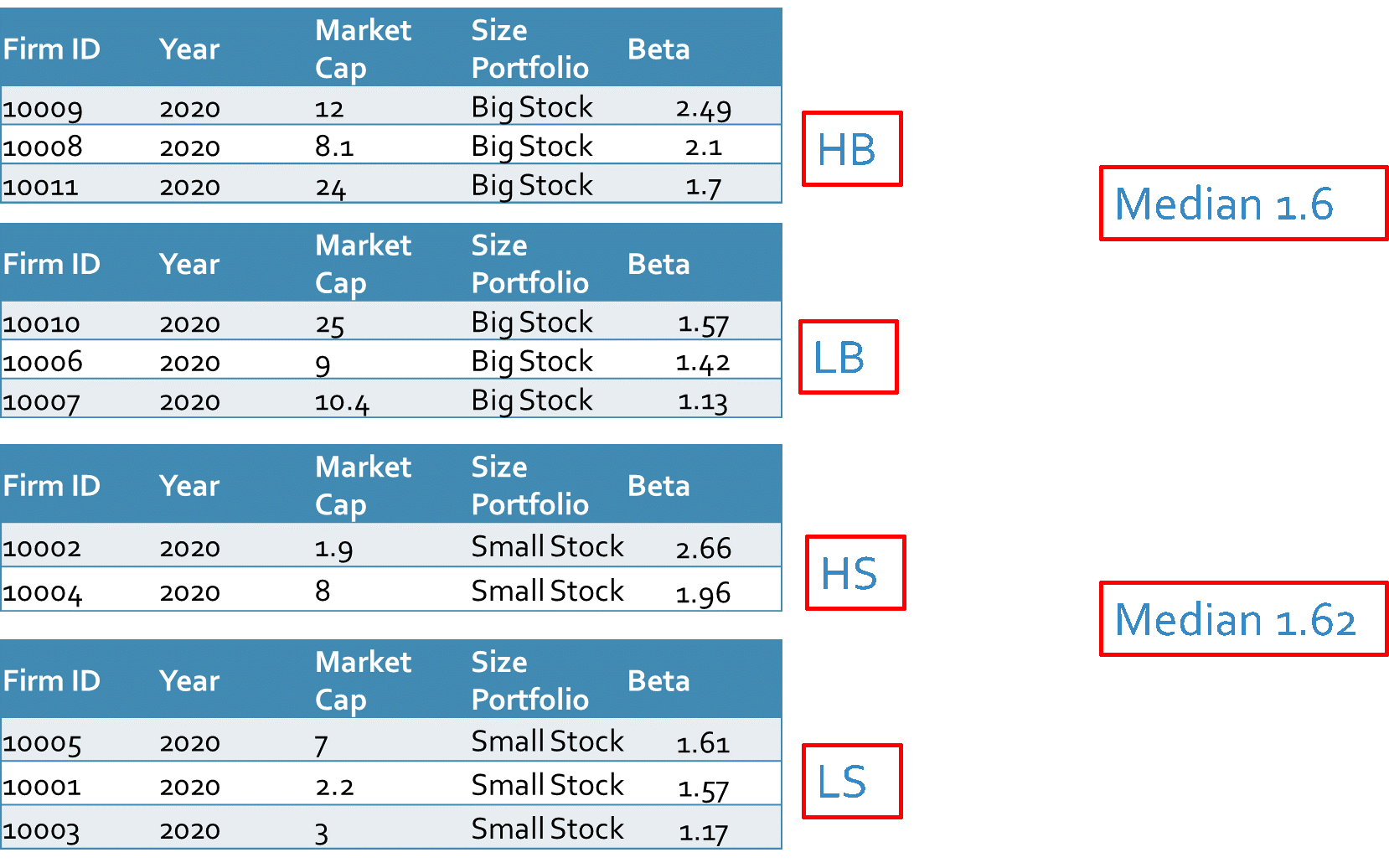
Example 2: Let’s take the same market capitalizations and the same firms as the previous example. In this example, we add the second factor (here Beta of the stocks) and then we sort the firms according to the median of size and median of Beta factors. The median of all Betas is 1.62, therefore, the firms with Betas greater than 1.62 have high Betas and the rest have low Betas.
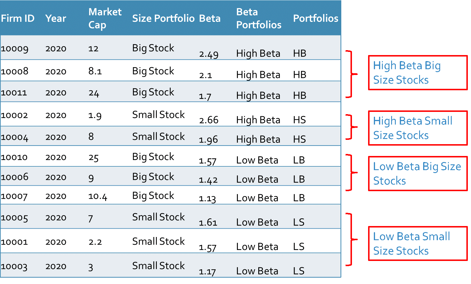
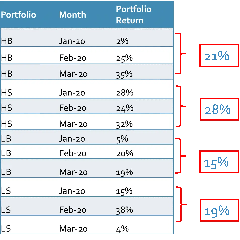
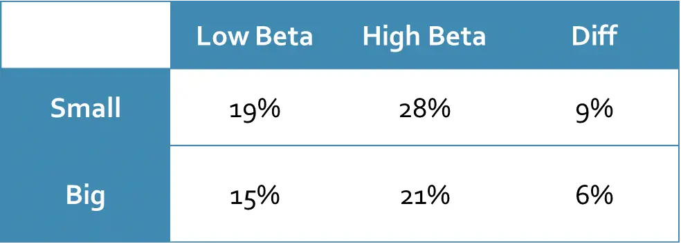
After integrating the stock returns, we can calculate the average return on each portfolio in the year 2020 as explained in the first example.
Dependent Sort
Now we want to introduce the second method of the bivariate model which is dependent sort. In this method, the breakpoints of the second factor are influenced by the first factor. So, it is important to know which factor to pick up as the first factor.
Example 3: Considering the same factors for the same period in example 2 we have two factors, and we start to sort the firms based on the size factor.
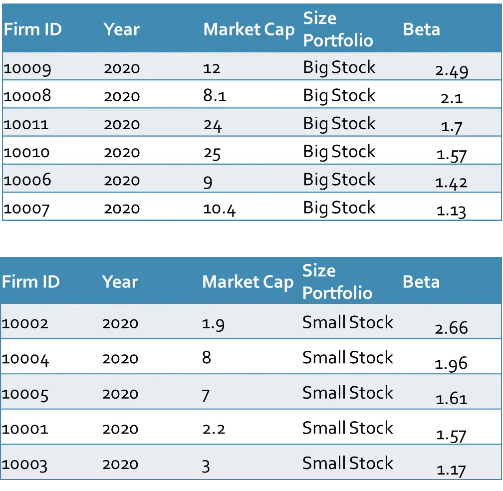
What we have done previously was that we sorted the firms based on the median of the Betas regardless of the size factor. But in this method (dependent sort) we calculate the median of the Betas within each size group and then sort the firms according to the median of the Betas in high and low within each size group. The following figure indicates the procedure more clearly.
Value Weighted Return
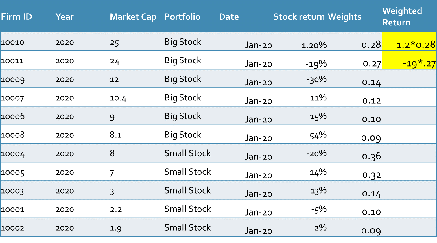
To calculate the value-weighted return of the portfolios we need the weights of each stock. This item is calculated by dividing the market capitalization of each stock by the sum of the market capitalization of all stocks within each group. Then we multiply each weight by its related stock return as it is done in the following table:
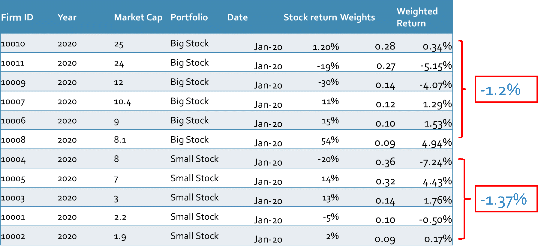
All that remains is to add these weighted returns together.
SMB and HML Construction
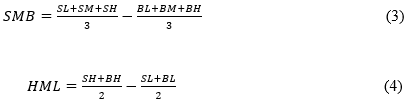
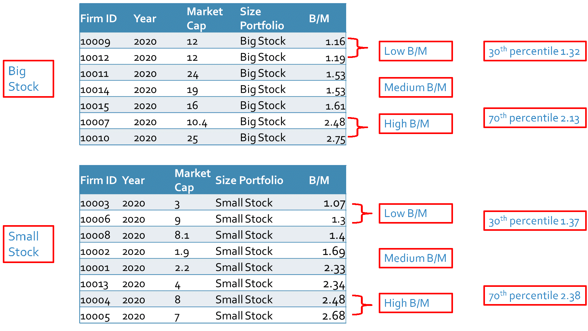
To construct the SMB and HML factors we need to download the market capitalization (closing price multiplied by outstanding shares) and book-to-market ratio of each stock from the database. Then we calculate the median of all stocks’ market capitalizations as our breakpoint to sort our stocks according to the size. The stocks with a market capitalization greater than the median are categorized as big stocks and the rest as small stocks. To group the stocks according to their book-to-market ratio we can use the 30th and 70th percentiles. The stocks with the top 30% of all book-to-markets are high-value stocks, the 40% in the middle are medium-value stocks and the rest are low-value stocks. Following this method, we get six portfolios (SL, SM, SH, BL, BM, and BH). After grouping the stocks, we can calculate the SMB and HML factors with the help of each portfolio’s average return according to equations (3) and (4).
Note: We are also allowed to use other percentiles (10%, 20%, 25%, etc.) or other metrics like mean, volatility, etc. to calculate the breakpoints for the SMB and HML factors. We should take into consideration that we have to use the same method for all years in the sample.
After learning how to calculate the factors and construct the portfolios, we are going to show in the next part, what exactly Fama and French did in their study in 1993. They used CRSP as their database which contains the U.S. companies in NYSE, AMEX, and NASDAQ. At the end of June of each year, they sorted all stocks based on the median of the market capitalization of stocks in NYSE.
The NYSE contains big stocks but the AMEX, and the NASDAQ stocks are usually small and medium. Therefore, the median is only caculated based on NYSE and applied on all stocks. If full sample is used to calculate median then the Big Stock portfolio will only contain stocks from NYSE and the Small Stock portfolio will contain stocks from AMEX and NASDAQ only.
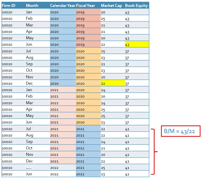
Furthermore, they needed the book-to-market ratio for each year to calculate the breakpoints for the value factor. Fama and French divided the book common equity for the fiscal year ending in calendar year t-1 by the market equity at the end of December of t-1. Whereas, portfolios are sorted in the June of year t. The reason why they constructed their portfolios with a lag of six months is to ensure that all the accounting data are available.
Example 4: In this example, we follow the Fama and French guidance and use the bivariate dependent sorting method. First, we sort all stocks based on the median of market capitalization in NYSE. Then we calculate the 30th and 70th percentile of the book-to-market of all stocks within each size group to sort the stocks.
In the next step, we calculate the value-weighted average return of each portfolio.
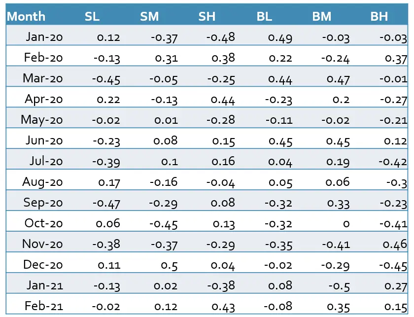
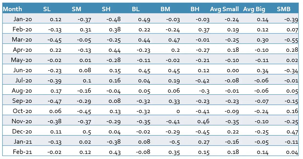
We calculate the SMB factor based on equation (3)
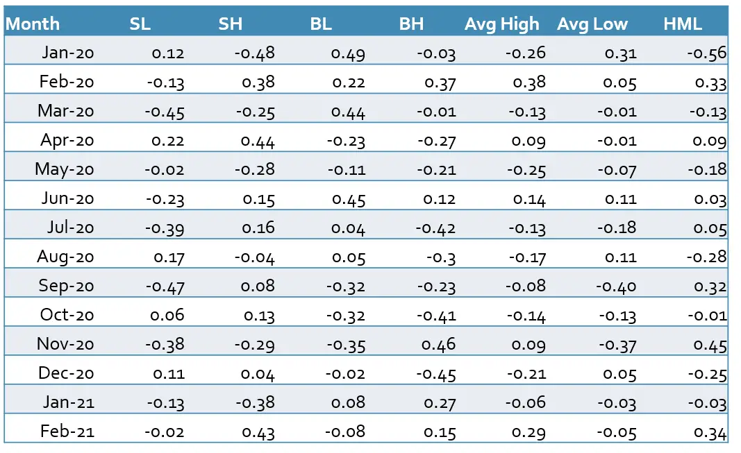
Finally, we calculate the HML factor as explained in equations (4)
In this blog we tried to give you a holistic understanding of the Fama and French study in 1933 and we hope that you enjoyed it.
In the next blog we will show you how you can replicate the FFM in Stata, R, and Python.