
Earning is one of the most important factors affecting economic decisions and the users of financial statements (stockholders and stakeholders). Users always pay special attention to accounting profit, therefore the users’ awareness of the reliability of earnings and profit can help them in making better decisions about profitability and analyzing financial statements. In preparing financial statements, managers use accounting procedures that provide the manager with a lot of flexibility to calculate profit, and in this regard, earnings management has been considered as one of the most important topics in accounting and finance.
What is earnings management?
Healey and Wahlen (1999) provide the following definition of earnings management: “Earnings management occurs when a manager uses his personal judgment for financial reporting with the purpose of misleading some stakeholders about actual economic performance or to influence the outcome of contracts that depend on the reported accounting figures.”
Accrual management is a type of earnings management, and it has two subcategories, namely Discretionary Accruals and Non-Discretionary Accruals.
Discretionary Accruals: That is, the management has authority over these accruals or the accruals manipulated by the management. Such as determining the useful life estimate in the subject of depreciation or determining the method of doubtful expenses.
Non-Discretionary Accruals: That is, the management has no authority over them and must act exactly according to the specific standards that have been set.
Most managers seek to manipulate discretionary accruals.
According to the explained content, it can be understood that the relationship between earnings management and other accounting items is very important. Additionally, in the financial literature, there is an assumption that there is a relationship between the management’s reporting decisions and the characteristics of the company’s information, and it assumes that earnings are the first sources of company-specific information.
To divided accruals into its two parts we have four models, according to past studies. These models are:
- Jones (1991)
- Dechow (1995)
- Kasznik (1999)
- Kothari (2005)
The formulas of these four models are as follows, and do note that all these models are used on panel data.
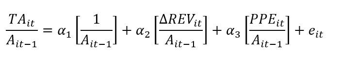
Jones (1991)
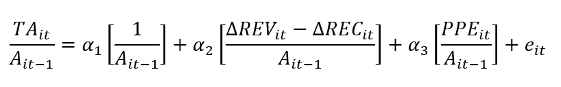
Dechow (1995)
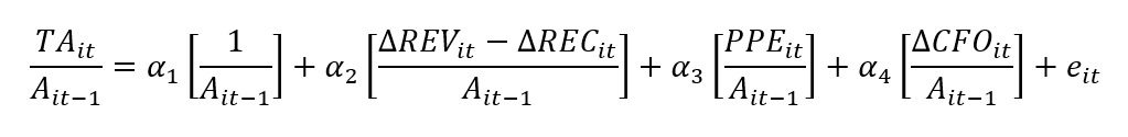
Kasznik (1999)
Kothari (2005)
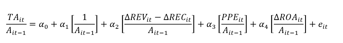
TA: Total Accruals Which is calculated as follows:
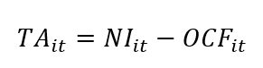
That means Net Income minus Operating Cash Follow.
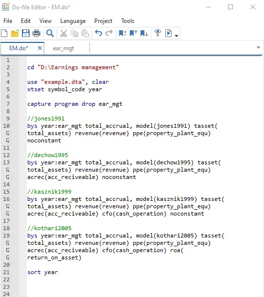
In each of the formulas above the error term is discretionary accrual and the fitted values from the above equation will become non-discretionary accrual. What we are going to do is run a regression for each of these models to get the coefficients. For the first three models we use noconstant option in Stata but for the last one the constant option. The procedure is declared stepwise as follows:
Step1: We should select a relevant model.
Step2: We calculate the variables required in the model.
Step3: We estimate a regression model. To perform the regression, we have two options. We can select either Pooled OLS (POLS) regression model or we can run cross-sectional regression for each year.
Step4: As mentioned earlier the residuals of the regressions are considered as discretionary accrual.
Step5: The fitted values from above regression become measure of non-discretionary accrual.
How to run a regression in Stata?
Firstly download the code from the following link:
Download Example FileFor performing the regression, you can use the following syntax in Stata:
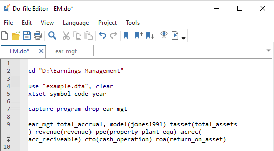
Instead of jones1991 you can write dechow1995 or kasznik1999 or kothari2005.
Remember: You cannot use ssc install to be able to perform ear_mgt, instead you can download the needed package from the following link:
After providing total_accrual you don’t need to divide it by the lag of asset, this will be done automatically by Stata.
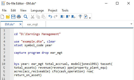
If you want to run cross-sectional regression for each year you can use the following code:
Jones (1991):
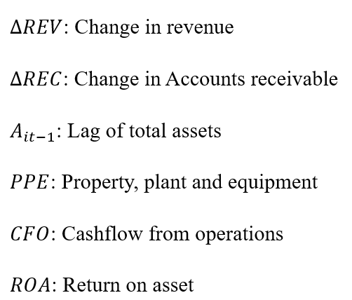
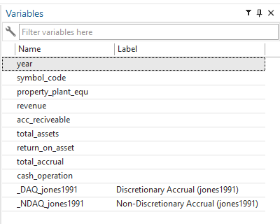
For Jones (1991) we need total accruals, total assets, revenue, and property, plant and equipment. After executing the syntax, two variables will be generated, their names start with DAQ and NDAQ. DAQ stands for discretionary accrual and NDAQ stands for non-discretionary accrual.
Dechow (1995):
In this model you should change the model to model(dechow1995) and add accounts receivable.
Kasznik (1999):
In this model you should change the model to model(kasznik1999) and add cash operations.
Kothari (2005):
In this model you should change the model to model(kothari2005) and add return on asset.
Note: Stata does not take cash operations into consideration, therefore, we don’t need to delete it.
At the end of the codes from Jone (1991) to Kasznik (1999)و you should add noconstant, but for Kothari (2005) it is not needed to add noconstant.
Following you can see the final codes in Stata:
Note: After executing the codes you can see that there are no values for DAQs and NDAQs in the first year, because we are using lag of total assets.