Estimate Multiple Regression In Stata

This article discusses how to perform multiple regression in Stata and how to deal with the results that are obtained. Unlike simple regressions that only have a single independent variable, multiple regressions have more than one independent variable.

Let’s start by loading Stata’s built-in auto dataset into Stata’s memory.

To run a multiple regression from Stata menu, the following menu options can be followed:

Statistics > Linear models and related > Linear regression

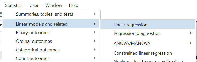
In the dialogue box that opens, choose the dependent and independent variables in the relevant fields from the drop-down menu. Note also that, on the title bar (the top most bar) of the window, Stata also mentions the command name that can be used to do the same operations from the command box. In this case, the command is simply regress.

Related Book: A Gentle Introduction to Stata by Alan C. Acock 

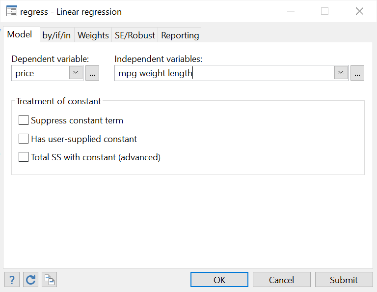
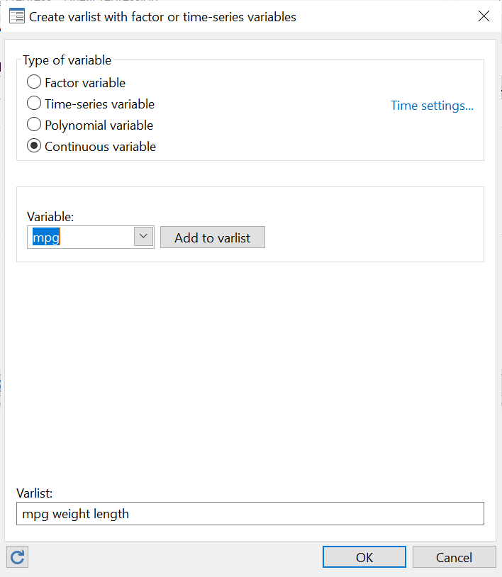
The little box with the three dots beside the drop-down menu can also be used to further choose more options and customize the regress command. In particular, these options are particularly important for independent variables. These are categorical (factor) or continuous or if you are dealing with time-series data.

For example, in our example, ‘mpg’, ‘weight’ and ‘length’ are continuous variables but ‘foreign’ is a dummy i.e. binary/categorical/factor variable. Let’s define them as so.

Note, in the following screenshot, that when adding categorical variables like ‘foreign’ to our varlist, they are added with an ‘i.’ prefix so that the variable in the regression looks like: i.foreign. This prefix indicates that it is a categorical variable. You can also define a base value, which is usually ‘1’ for a binary variable. But you can choose a relevant one from the list of options provided.

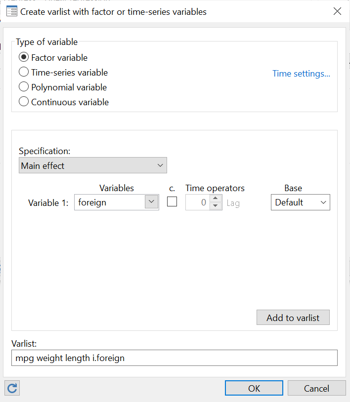
Click ‘OK’ on this window, and then ‘Submit’ on the main regress window. The multiple regression will be run with the following output produced:

Interpreting Multiple Regression Output in Stata

Let’s go over what this table tells us.

The ANOVA Table

Related Article: How to Perform the ANOVA Test in Stata

The upper left corner that displays the Model and Residual sum of squares (SS) is the ANOVA table.

Number of Observations in a Multiple Regression in Stata

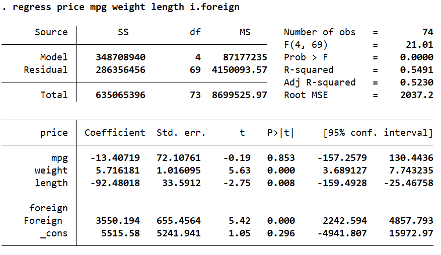
Beside it, on the right, are some statistics that give a summary of the overall regression. The number of observations used in this regression were 74. This number might sometimes differ from the actual number of observations in your data if you are using if conditions or if there are some missing observations for the regression variables (casewise deletion).

F-Stat in a Multiple Regression

F(4, 69) represents the F-stat, which indicates the joint significance of our model. This significance can be ascertained by the p-value, Prob > F provided under it. Because this p-value is less than 0.05 (it is 0 in our case), we can say that our model is indeed jointly significant.

R-Squared in a Multiple Regression

The R-squared value represents the amount of variation in the dependent variable that is explained by the independent variables. In this regression, 54.9% of the variation in ‘price’ is explained by the four independent variables we added in our model. The remaining variation in the dependent variable ‘price’ can be said to be due to the variables that we have not added in our model. Generally, as a rule of thumb, an R-squared value of less than 0.21 (21%) is considered to be weak, but anything above 0.31 (31%) is considered strong. Many times, though, the R-squared alone is not considered that important to evaluate the suitability of a regression. Often, this value is quite low, but the regression is considered valid. Whether the R-squared value matters, or not, depends on the context and application.

Adjusted R-Squared in a Multiple Regression

The Adjusted R-squared is a representation of how much a new variable improves our regression model. This value goes up if a new independent variable improves the model but goes down if the model is not improved as expected. This value is always less than the first R-squared value. A high number of independent variables and a low number of observations generally results in a higher Adjusted R-squared value.

Interpreting Coefficients in a Multiple Regression in Stata

Let’s interpret the bottom part of the table that represents the relationships between the dependent and independent variables.

The very first column has the names of your independent variables.

The second column titled ‘Coef.’ displays the corresponding unstandardised regression coefficients for these variables also known as the beta coefficients or the coefficient estimates. These coefficients represent the change in the dependent variable, ‘price’, for a 1 unit change in the independent variable. For example, here, when the mileage (‘mpg’) of a car goes up by 1, the price of that car decreases by $13.4. The decrease is indicated by the negative sign. Conversely, if the weight of a car goes up by 1 lb, the price goes up by $5.72. In the case of the length of a car, a 1 inch increase in length leads to a decrease of $92.48 in its price.

‘_cons’ is the intercept term, also called the alpha value or the constant.

In regressions of other kinds, these coefficients can also display the probabilities, odds ratios and other statistical measures of change.

The third column represents the standard errors associated with these coefficients.

Related Article: Using Putexcel to Export Stata results into Excel

Hypothesis Testing in a Multiple Regression in Stata: t-stat and p-value

The next two columns titled ‘t’ and ‘P>|t|’ are columns that help us with hypothesis testing. They help us determine whether a coefficient is statistically significant or not. The t-stat is obtained by dividing the coefficient with its standard error. The null hypothesis that we use these stats for is typically that the coefficient is equal to zero, or,alternatively that the coefficient is statistically insignificant.

• If the t-stat is greater than 1.65, we can safely reject the null hypothesis of there being no relationship between the dependent and independent variable at the 10% significance level. That is to say, the coefficient is significant at the 10% level.
• A t-stat value between 1.65 and 1.96 indicates that coefficient is significant at the 5% significance level.
• A t-stat equal to or above 2.58 indicates that coefficient is significant at the 1% significance level.

An even easier check is the p-value (‘P>|t|’).

• If the p-value is less than 0.01, it can be rejected at the 1% level of significance.
• If it is less than 0.05, we can reject the null hypothesis at the 5% level of significance.
• If it is less than 0.1, the null can be rejected at the 10% level of significance.

When these criteria are not met (depending on our choice of the significance level), we fail to reject the null hypothesis (that the coefficient is zero ) and say that the coefficient is statistically insignificant.

In social sciences, a significance level of 5% or 10% is acceptable, but in fields like medicine where more accuracy and surety is required, a 1% significance level is favoured when ascertaining the statistical significance of a regression estimate.

In this table, the p-value of ‘mpg’ is 0.853 which is very high and beyond any levels of significance described above. Based on this regression, it is thus statistically insignificant, and we fail to reject the null hypothesis that there is no statistically significant relationship between ‘mpg’ and ‘price’. In other words, the coefficient can be said to be zero indicating there is no relationship between the mileage and price of a car.

‘weight’, ‘length’, and ‘foreign’ (a categorical variable) are statistically significant. Note that for ‘foreign’ the coefficient is interpreted for the category which is equal to 1 which in this case is the category representing foreign cars. Coefficients for categorical variables are interpreted in comparison with the category that is equal to 0. In this example, we can say that as compared to domestic cars (‘price’==0), foreign cars have a price that is higher by $3550.194

There are two types of hypothesis: directional and non-directional. The tests we discussed above fall under non-directional hypothesis. By default, Stata does a two-tail test when reporting the t-stats and p-values in a regression table.

Confidence Intervals in multiple regression in Stata

The probability of a coefficient falling in a given range is given in the last column titled, ‘[95% Conf. Interval]’. A confidence interval is the mean of our coefficient plus/minus the variation in that coefficient. The value of 95% indicates that 95% of the values for our coefficient estimate will fall within two standard deviations from the mean.

For the purposes of hypothesis testing, if the p-value is less than 0.05, i.e. the coefficient is statistically significant, then the null hypothesis value (usually 0) should notfall in the 95% confidence interval.

The confidence interval for the ‘mpg’ coefficient is -157.2579 and 10.4436. The value of 0, falls in this interval, again indicating that it is not statistically significant.

Note that ‘weight’, ‘length’, and ‘foreign’ are all statistically significant. Their p-values are less than 0.05 and their 95% confidence intervals do not include 0.

Standardizing Coefficients

Based on the unstandardised coefficients reported in the table, we cannot ascertain whether one independent variable has a higher effect on the dependent variable than another. Here, for example, we cannot quite tell whether ‘weight’ has a bigger effect on ‘price’ or ‘length’.

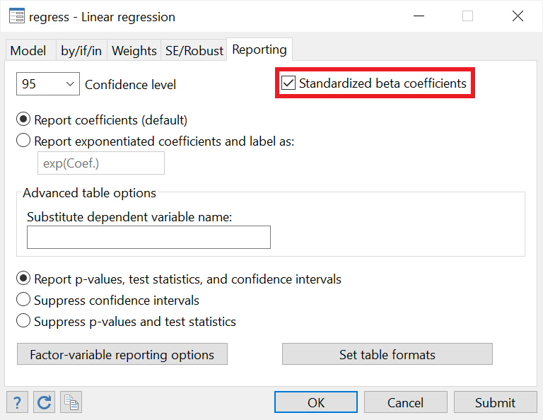
We can report standardised beta coefficients in a regression by going back to the ‘Reporting’ tab in our regress window, and checking the option called ’Standardized beta coefficients’

To alter the regress command to report the standardised coefficients, we simply add the option beta. In the last column, we see that the standardised beta coefficients are reported.

Related Article: Correlation Analysis in Stata (Pearson, Spearman, Listwise, Casewise, Pairwise)

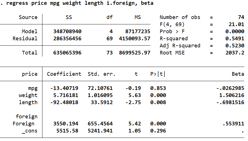
While unstandardised betas are scale dependent (i.e. their range and distributions differ) and do not tell us the relative contributions of each variable on the dependent variable, standardised beta coefficients allow us to see which variables have a bigger or smaller effect relative to others. These betas are obtained by dividing the unstandardised coefficients by their standard deviations. The standardised betas have a mean value of 0 and a standard deviation of 1.

We can clearly see that ‘weight’ has the highest impact on ‘price’ as compared to the other independent variables.

Standardised beta coefficients are interpreted slightly differently than unstandardised coefficients. We say that for a 1 standard deviation change in, say, ‘weight’, the ‘price’ goes up by 1.5 standard deviations. 

This interpretation gets slightly tricky and problematic for categorical variables. We cannot talk about a 1 standard deviation change in the variable because categorical variables are not continuous.

A better approach to see the individual contribution of a categorical variable on the dependent variable is to look at the change in the R-squared value when the categorical variable is added to the regression. You can do this for all variables. Try regressing ‘price’ on just ‘mpg’. Then in a second regression, add ‘weight’, and see the increase in R-squared. This change will indicate how much of the variance in ‘price’ is uniquely explained by this new variable. Keep adding variables one by one and note the change in R-squared. This is called increment in R-squared or partial/semi-partial correlation.

Partial and Semipartial Correlation

Stata can report these partial and semipartial correlations through the pcorr command as well. The pcorr command is followed by all the variables that we included in our regression.

This command displays the partial and semipartial correlation coefficients of a variable with the dependent variable after the effects of the rest of the variables are removed.

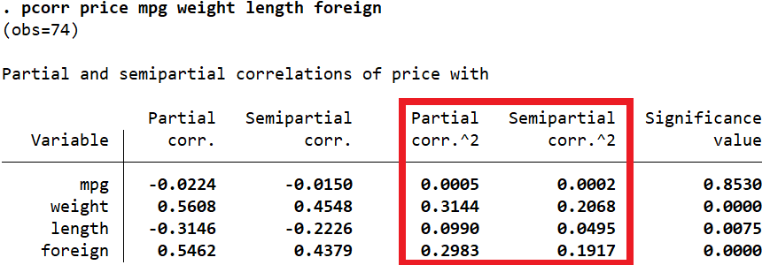
We are interested in the third and fourth columns: ‘Partial corr.^2’ and ‘Semipartial corr.^2’. The latter, ‘Semipartial corr.^2’, represents the change in R-squared when that variable is added to the model. 

Like the standardized coefficients, this table also shows that ‘weight’ has the highest effect on ‘price’ relative to other variables (Semipartial corr.^2 = 0.2068). The value means that when ‘weight’ is added to the regression, the R-squared goes up by 0.2068 or 20.68%. Alternatively, 20.68% variation in ‘price’ is explained by ‘weight’. The very last column also indicates that this change in R-squared is statistically significant (p-value = 0.000) and therefore, we can say that ‘weight’ is a statistically significant predictor of the price of a car.