
This article will talk about correlations – how they can be obtained in Stata, their various types, various interpretations, Pearson and Spearman correlations, listwise (casewise) and pairwise deletion, and some other concepts pertaining to correlations.
Download Example FileCorrelation is simply defined as the association/relationship between two variables. For example, an education can have a positive correlation with one’s wages (when one increases, the other also increases, and vice versa); while an increase in exercise may be correlated with a decrease in weight (negative correlation).
When talking about correlations, we do not refer to variables as ‘independent’ or ‘dependent’ variables. These are terms that we use when running regressions where the effect of one or more independent variables is being studied on one dependent variable. Correlation is simply a two-way relationship between two variables. The correlation coefficient tells us the strength (i.e. the magnitude) and direction (positive or negative) of the association/relationship between the two variables.
The higher the absolute value is of the correlation coefficient, the stronger is this relationship. Typically, absolute values between 0 and 0.3 are considered weak correlations, 0.4-0.5 are considered moderate, while anything between 0.6 and 1 is treated as a strong correlation. Davies (1971) proposed the following descriptions of for different (and absolute) values of the correlation coefficient though usually it is enough to just categorise them into weak, moderate and strong.
| r | Adjective |
| 1.00 | Perfect |
| 0.70-0.99 | Very High |
| 0.50-0.69 | Substantial |
| 0.30-0.49 | Moderate |
| 0.10-0.29 | Low |
| 0.01-0.09 | Negligible |
Unlike regressions, correlation does not indicate causality. Well setup regressions give us the causality between two variables where we can safely deduce that on average, a change in the independent variable will lead to a certain degree and direction of change in the dependent variable. Correlation is only illustrative of how two variables move together. For example, a scatterplot of one’s science scores and math scores may show us that as science scores increase, math scores also increase i.e. they tend to move together. This says nothing about the causal impact that either of these scores have on each other.
The dataset we will use for this article is the ‘high school and beyond dataset that can be loaded via the following command:
use https://stats.idre.ucla.edu/stat/stata/notes/hsb2
This is a dataset about students with variables pertaining to their gender, race, and certain academic indicators.
Related Article: How To Make Heatplot In Stata | Correlation Heat Plot
Pearson Correlation
The correlate command in Stata returns us the Pearson correlations typically used with continuous variables.
Correlation from Menu
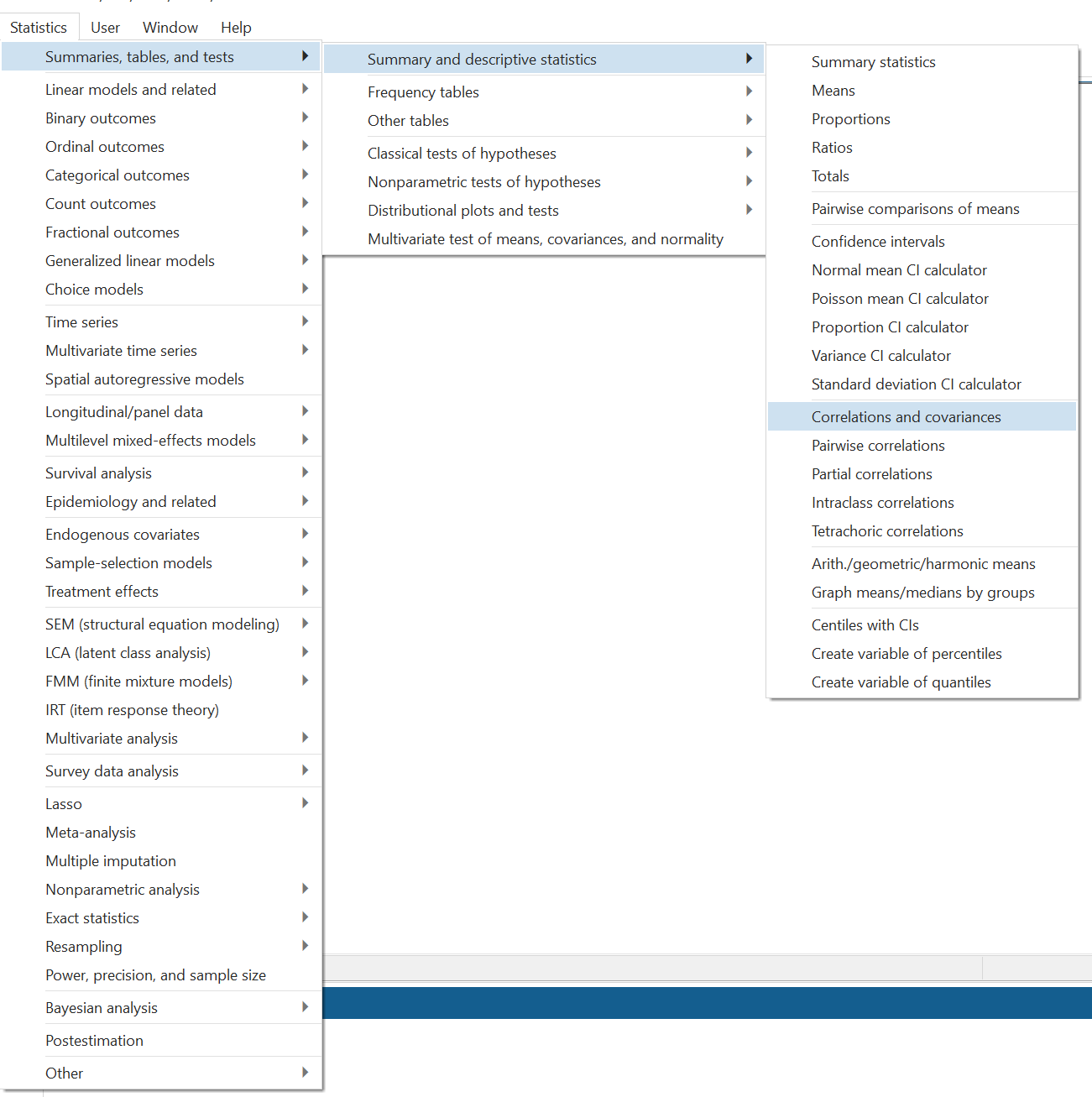
Before we get into the commands, let’s see how we can obtain correlations in Stata via the menu.
Statistics > Summaries, tables, and tests > Correlations and covariances
In the dialogue box that opens, choose a list of variables. We choose the following seven variables:
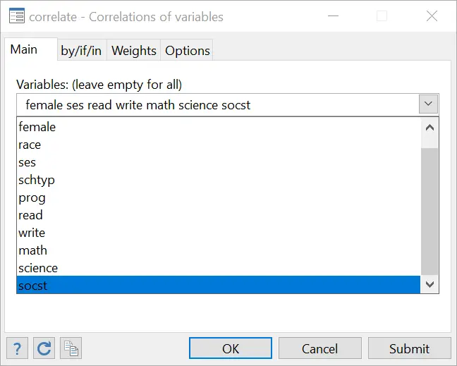
Stata will then return a covariance table that displays the covariances of each of these seven variables with each other.
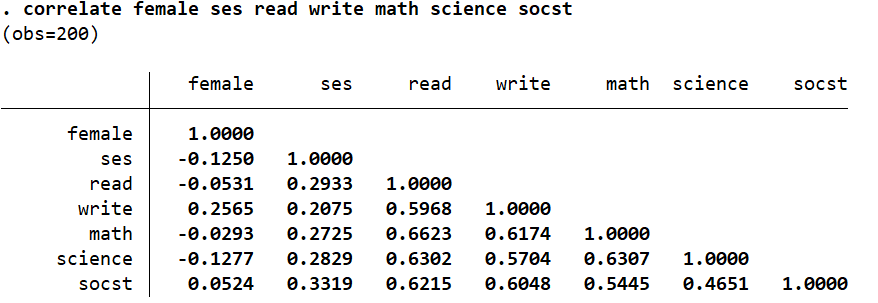
Remember that the correlation of a variable with its own self will always be 1. The correlation between gender (‘female’) and science scores (‘science’) is a very weak -0.1277 whereas, the correlation between math scores (‘math’) and reading skills (‘read’) is a very high 0.6623. The score of 0.461 between the social studies score (‘socst’) and science score (‘science’) is a moderate correlation. The correlation between ‘female’ and ‘read’ is a negligible -0.0531.
Categorical Variables and Correlations
In this dataset, ‘female’ is dummy/categorical variable. It is equal to 1 if a student is a female, and 0 if they’re a male. In light of this, the correlations of ‘female’ would be interpreted accordingly with respect to the categories the variable. Whenever the value of ‘female’ is 1, science scores tend to go down (as illustrated by a negative, but weak correlation of -0.1277). Alternatively, female students are (weakly) associated with lower science scores relative to male students. The magnitude of correlations of ‘female’ with all other variables suggest that being a female is not strongly or even moderately associated with any of these variables.
The variable ‘ses’ which describes the socioeconomic status of each student has three categories. The codebook ses command lists these categories (or alternatively we can use tabulate ses to get the list of categories):
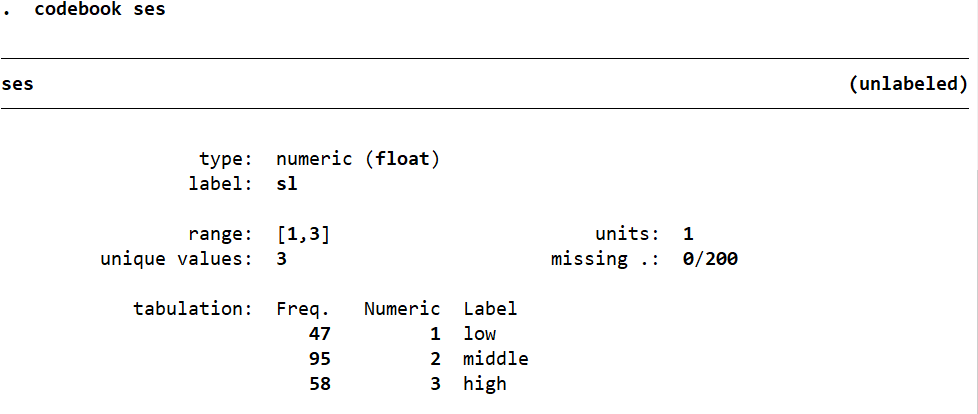
A value of 1 is assigned to those from a low socioeconomic class, 2 for those belonging to the middleclass, 3 for those from the high socioeconomic class.
The correlations are interpreted accordingly to. As the value of ‘ses’ increases, i.e. the higher a student’s socioeconomic status gets, their scores for all the components listed also go up. The highest of these correlations is 0.3319 with the social studies score (‘socst’) which is a moderate correlation at best.
Certain variables like ‘race’ do not have any such levels so it becomes tricky to find a correlation between one’s race and academic scores in such a dataset. One may address this by creating dummy variables for each race and studying their correlations with the academic variables.
Related Article: Publication Style Correlation Table in Stata
Listwise/Casewise Deletion
The correlations calculated above were done using what is known as listwise or casewise deletion. Here, Stata omits from calculations those observations/cases where any missing value exists. We can check how many observations/cases Stata used when it estimates the correlation table after the correlate command by running:
return list
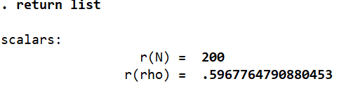
Note that this command will be run right after the correlate command. In this case, Stata is calculating the correlations using the full set of 200 observations that the data has. This is because there are no missing values for any variable in this dataset.
To see what happens when there are missing values, lets create some at random by editing this dataset. This can be done so by pressing the Data Editor button on the task bar, and then manually tying in any changes in the window that opens.

Alternatively, you can also use commands given below to make changes to the data. For example:
replace read = . in 2 replace read = . in 10 replace read = . in 22 replace write = . in 18 replace math = . in 26 replace science = . in 30 replace science = . in 16
The above commands will generate 7 missing values in our current dataset so that we can demonstrate how casewise deletion works. Let’s rerun the correlation command.
correlate read write math science ses female
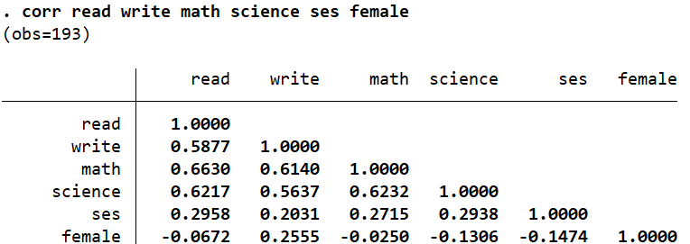
These values are different from the ones we obtained previously because we have made some changes to the dataset. Let’s run the return list command again and see what changed.
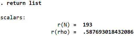
We can see that Stata only used 193 observations when creating the correlation table above whereas the dataset still has 200 observations. This is because it omitted the 7 observations from calculations that carried a missing value for some variable.
Casewise deletion leads to a few problems. Firstly, it reduces the sample size that the correlation calculations are done on. Secondly, this in turn, may indicate the presence of a bias. In our example, students who scored low may be reluctant to share data about their grades. In this manner, the sample and any subsequent analysis done will be more heavily skewed towards those with higher grades. (Similarly, people are often reluctant to share their salaries if they are too high or low). To counter this, we ask Stata to perform what is called the pairwise deletion.
Related Book: Basic Econometrics by Damodar Gujarati
Pairwise Deletion
In the case of pairwise deletion, Stata uses all available observations for a pair of variables to calculate a correlation coefficient for them even if other variables for the same observations are missing. For example, observation number 2 may have a missing value for ‘read’. Stata will not omit this observation for every calculation. It will obviously omit it when calculating the correlation of ‘read’ with other variables, but observation number 2 will not be ignored when correlations are being calculated for, e.g. ‘write’ and ‘math’, ‘science’ and ‘socst’ and so on.
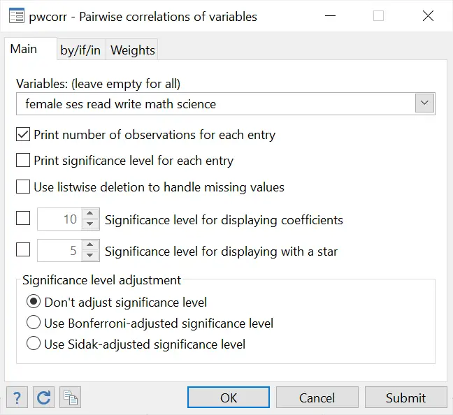
Pairwise correlation can be calculated via the following menu path:
Statistics > Summaries, tables, and tests > Pairwise correlations
In the dialogue box that opens, choose your desired list of variables as before. Also check the very first option under the variable field which tells Stata to “print number of observations for each entry”.
A table of correlations is produced as before, but this time, it also shows the number of observations that were used in the calculation of each correlation coefficient.
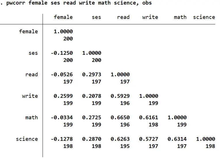
Because there are no missing values for ‘ses’ and ‘female’, the full set of 200 observations is used. Because there is one missing value for ‘write’, and three missing values for ‘read’, it omits these four observations but only while calculating this coefficient (196 observations used).
You can also see that the command for obtaining pairwise correlation is pwcorr, and the option used to display the number of options for each correlation coefficient is obs. The command used to produce the table above is:
pwcorr female ses read write math science, obs
Also note that in the dialogue box that opens, there is also a third option to ‘use listwise deletion to handle missing values. This produces correlations exactly similar to the correlate command. The number of observations would, in this case, be the same for all correlation coefficients. You can also run the following command for this:
pwcorr read write math science ses female,obs listwise
You can also check the second option that lets Stata ‘print significance values for each entry’.
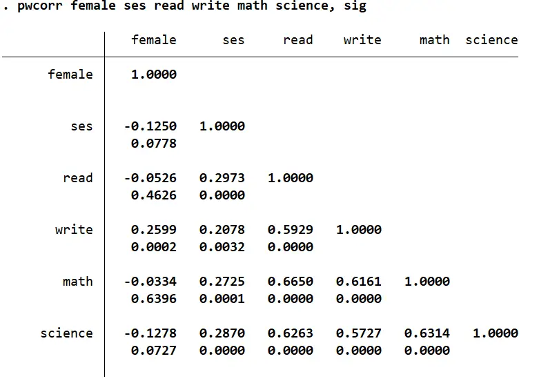
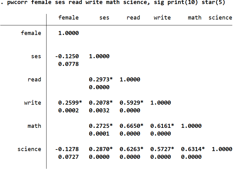
The significance levels are reported under the correlation coefficients. Anything below or equal to 0.05 shows a significant correlation. You can also get this by using the pwcorr command with the sig option:
pwcorr female ses read write math science, sig
Statistical Significance vs. Substantive Significance
A concept worth understanding at this point is the difference between statistical significance and substantive significance.
A correlation has substantive significance if the ‘r’ (the correlation coefficient) is moderate or strong i.e. greater than 0.3 in absolute terms
Statisitcal significance is illustrated by the p-value – the values we just reported above using the sig option. Any p-value less than or equal to 0.05 would be considered statistically significant.
A substantive significance does not imply statistical significance and vice versa. For example, the correlation between ‘ses’ and ‘write’ is not substantive (r = 0.2078), but it is statistically significant (p-value = 0.0032).
The higher the number of observations, the more likely it is for a correlation to be statistically significant.
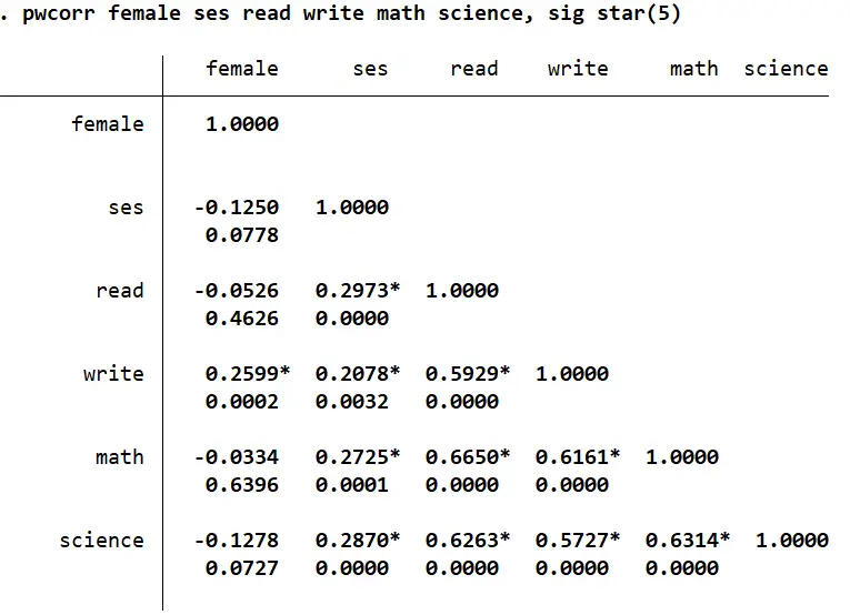
We can also tell Stata to indicate the statistical significance using asterisks. This can be done by checking the box which lets you set a significance level to display asterisks/starts.
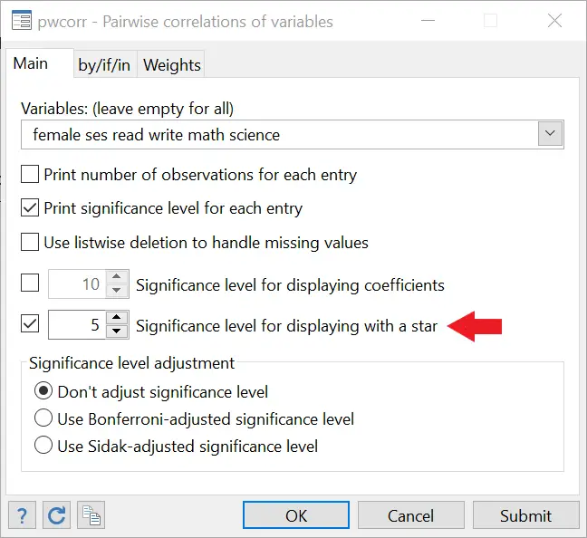
An asterisk is now displayed alongside correlations that are significant at the 5% significance level. The accompanying command for this is:
pwcorr read write math science ses female,sig star(5)
The option above this, ‘Significance level for displaying coefficients’ does not display correlation values that are not significant.
The option for this is print()
pwcorr read write math science ses female, print(10)
Bonferroni and Sidak Adjustmed Significance Levels
If, say you were interested in correlations as a whole, you would have to make some adjustments to the significance levels being reported. The Bonferroni adjustment corrects the p-values to address the risk of a type 1 error (rejecting the null when it is true i.e. treating a correlation as statistically insignificant when it actually is significant). A similar correction is called the Sidak adjustment.
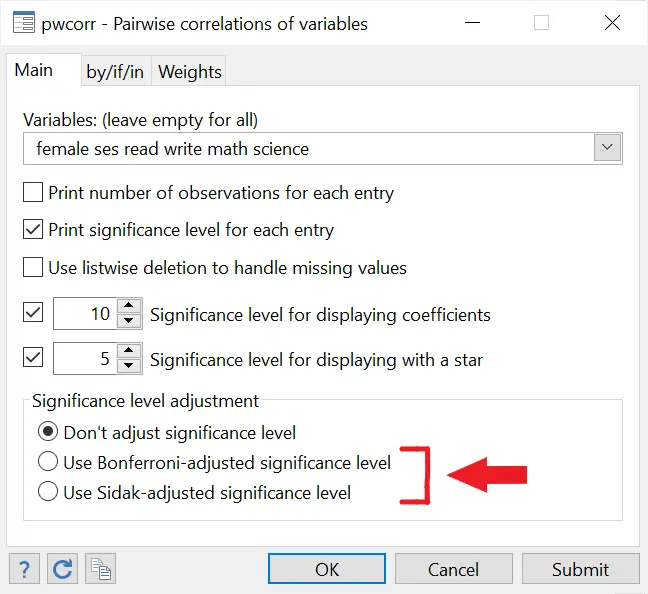
Both these adjustments may be made using the last two options in the dialogue box. The accompanying command for Bonferroni adjustment is:
pwcorr read write math science ses female, sig bonferroni
Spearman Correlation
Spearman correlation comes in handy when there are influential or outlier values in our data that may skew our correlation analysis in one direction or another. Rather than use the original continuous values of the variables, Spearman correlation ranks the data and then calculates correlation between variables. Let’s load Stata’s automobile dataset for this example.
sysuse auto.dta, clear
We are interested in the relationship between the ‘price’ and ‘weight’ variable. Let’s replicate the ‘ranks’ that Spearman correlation uses by generating two new variables that rank the observations based on their ‘price’ and ‘weight’ values.
egen rprice=rank(price) egen rweight=rank(weight)
Let’s do a simple correlation between ‘price’ and ‘weight’.
corr price weight
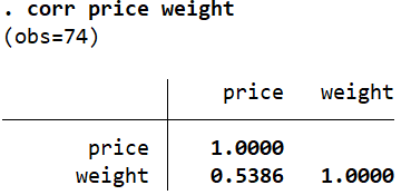
This correlation of 0.5386 is quite high because certain prices have influential values that skew this correlation upwards.
Let’s now run the correlation between the ranked variables we created.
corr rprice rweight
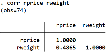
This value is slightly lower as it adjusts for the presence of ordinal/influential data. The above activity where we created ranked variables illustrated how Spearman correlations are calculated. If we run the spearman command directly, we will obtain the same correlation as we did above between our ranked variables, i.e. 0.4865.
spearman price weight
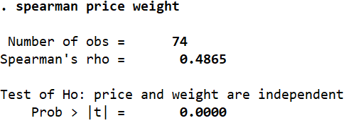
Once again, the same positive and moderate correlation of 0.4865 is reported.