
In Stata, you can make graphs and edit them as per the requirements of data. Apart from creating graphs, you can also combine multiple graphs using the different techniques. To visualize this, import a data set using the following command:
Download Example Fileuse "combine graphs.dta",clear
For combining multiple graphs, the imported data can be used for the demonstration. As evident from the data window, there are two types of variables in the data. These variables are continuous and categorical variables. The continuous variables include wage and hours, the categorical variables, on the other hand, include race and marriage.
To make the bar chart or graph of a certain variable over another variable, apply the following path
Graphs > Bar Chart
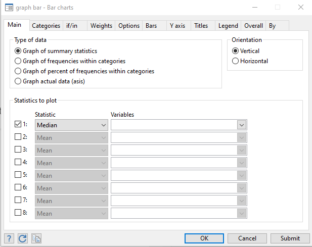
A new window will appear, select “median” in statistics and select “wage” in variables drop down menu. Then click on the categories tab and in group 1 select the race variable. Click ok if you wish generate bar graph
This generates a Bar chart based on variable wage over race. It means that you need a graph where you want to see the wage of different groups, based on their race. The statistics you chose is based on your requirements. For example, if you want the graph to be based on average of wage, you would choose the option of mean. Similarly, if requirement asks for median of race, the median option will be chosen from the statistics.
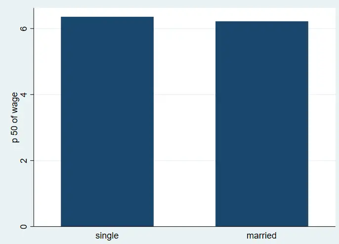
Similarly, if we want the bar chart based on median of wage over married, we will use the following command:
graph bar (median) wage, over(married)
The following graph will be created
Related Article: How to Create A Histogram in Stata
Similarly, we can get the bar chart of wage over race by using the following command
graph bar (median) wage, over (race)
The above command will generate the following graph

Naming Graphs while combining multiple Graphs in Stata
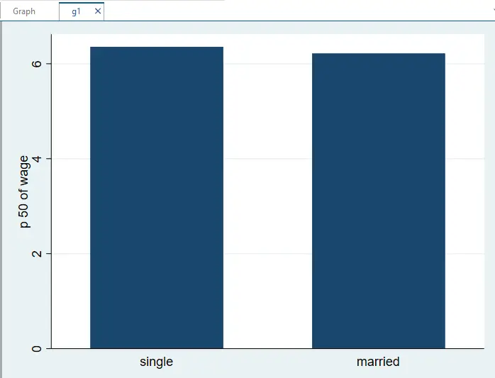
The graphs above generated are replaced as quickly if we don’t name them separately. For instance, the graph we made using the first command will be replaced by the graph of second command because we didn’t specify the names for graphs. So to prevent graphs from being replaced by the new command, it’s important to name them. To name a graph, let’s say g1, use the first command, with specifying the name of graph.
graph bar (median) wage, over (married) name(g1, replace)
The following graph will be generated with the name of g1.
Related Article: Scatter plots in Stata
Now, to create another graph, use the second command used above and name it g2.
graph bar (median) wage, over (race) name(g2, replace)
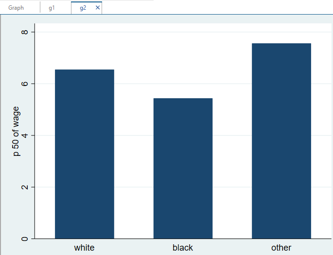
As evident from the image, the graph generated above didn’t replace the first graph, and is named as g2.
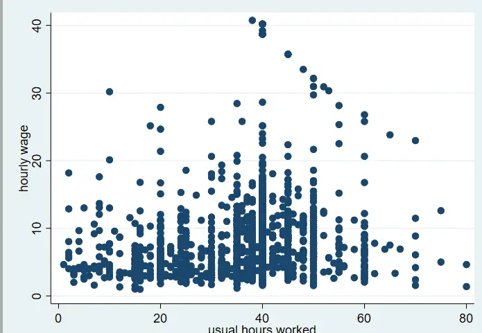
If we wish to create a graph other than bar graph, say a scatter plot, we can create scatterplot graph too using the following command:
twoway (scatter wage hours, sort ), name(g3, replace)
The following graph of scatter plot will be generated using the above command.
Access graphs stored in memory
Naming graphs doesn’t save graphs in hard disk or in your PC. These graphs are just stored in Stata memory. If we need to look up graphs saved in Stata memory, the directory of Stata will be opened. Use the following command to open Stata directory
graph dir
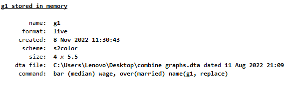
The above command will lay out all the details of the available graphs in Stata Memory. For instance, in this case we have three graphs named g1, g2 and g3 saved in directory. If we have to get the all the details of the graphs, including the date it was created and the command by which the graph was generated, we will use the following command:
graph describe gr
The following details will be available against the graph g1.
Related Book: A Visual Guide to Stata Graphics by Michael N. Mitchell
Combine multiple graphs
To combine the two graphs, preferably the same type of graphs i.e. bar charts, we will use the command graph combine along with the names assigned to those graphs.
graph combine g1 g2
A new graph will be generated which has two graphs g1 and g2 that were needed together.
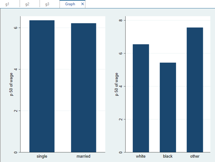
Now as we can see from the above graph that we have same variable on y-axis that is wage. So if we combine both graphs and keep the same axis common, it would be easier to analyse the graphs based on different independent variables (x-axis) overdependent variable (y-axis).
To combine two graphs keeping the common axis, use the following command
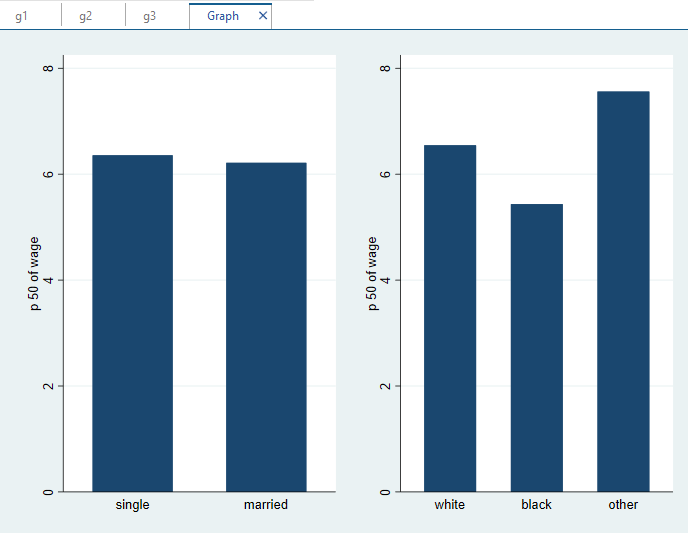
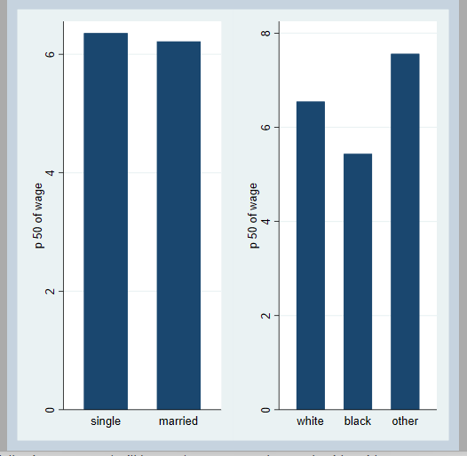
graph combine g1 g2, ycommon
Now the graph generated has same variable on y-axis i.e. wage and different variables on x-axis.
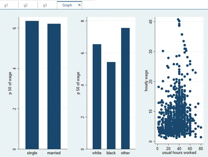
We can also stack x and y-axis, and can have them stacked over the one another. However, if we want to stack columns together and rows together, we can use the commands to keep the columns we want to keep and the rows we want to keep together. So if we want to keep column 1 and stack the graphs 1, 2 and 3, we can get one single graph containing columns only. The following command will be used to combine columns and stack graphs together
graph combine g1 g2 g3, col(1)
The following graph will be generated.
Similarly, if we want to keep rows only in the graphs and stack graphs together, we will use the following command
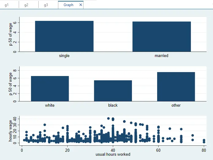
graph combine g1 g2 g3, row(1)
We will get the following graph
The hole Option
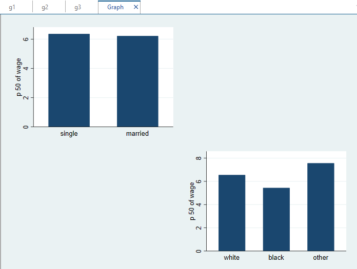
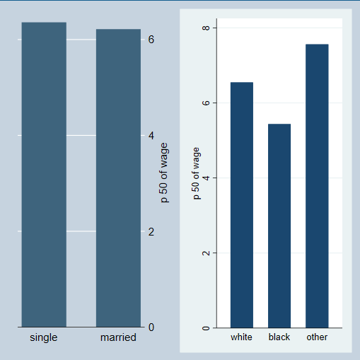
In Stata, while dealing with graphs, we can also use the hole option. What this hole option does is, it creates an empty space in the graphs window, giving user an option of either to add a new graph in the window or write something. For instance, in the following image, we have three graphs, and there is empty space at the right bottom side of the window. As we can see, the window is a 2 × 2 matrix, so if we want to keep graphs 1 and 2 in such way that, there is empty space at 22nd and 3rd place in the matrix. To get such kind of matrix, we will use the following command
graph combine g1 g2, hole(2 3)
The following matrix will appear
Similarly, we can use any other combination of space that we want to be appeared empty in the matrix.
Shrink the text:
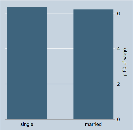
The text of the graphs can be shrinked using the command altshrink. The altshrink command specifies alternative ways to determine size of the graph, including its thickness, markers and size of the text. Using the following command, the text of the graph can be shrunk in Stata
graph combine g1 g2, altshrink
Although the new text would not be much different from the original graph, there exists difference in text from the previous graph.
Now, as we have combined the graphs previously, but these graphs are not distinguished. For instance, if we want to combine graph 1 and graph 2, the combined graph will have name Graph. But if graphs 3 and 4 are also to be combined, the name of that graph too will be Graph. So to distinguish the grouping of graphs, we can combine these graphs and give them a unique name. To assign a certain name to these graphs, following command will be used
graph combine g1 g2, name (original)
Now the combined graph has a name, called “Original”.
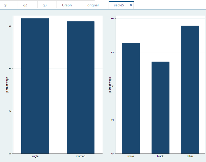
We can also change the text of a graph to a certain size. If the graph text is supposed to shrink by 0.5 or half of the original size, it can be done using the following command:
graph combine g1 g2, iscale(0.5) name(scale5)
The text of the graph will shrink to half of its original size, as evident from the following image.
Similarly, the size of text can be changed by 0.5 points or by whatever point you want to increase by using the same command used above, however changing the 0.5 size to 1.5 in the command. Note that while increasing the text to 1.5, we will use the asterisk sign in command to instruct Stata as to mention to compare the new graph with the previously combined graph.
graph combine g1 g2, iscale(*1.5) name(scale15)
The new graph generated with a name of scale15 will have text size of 1.5.
Graph Stored on hard drive
Graph generated in Stata are usually stored in Stata memory, however these graphs can also be stored in the hard drive of the computer. To save graphs in hard drive, write the name of the generated graph, and the name by which you want your graph to be saved and use the replace option, as if there already exists a graph with this name, this graph can replace it.
The following command will be used to save graph in hard drive of the computer.
graph save “g1” “g1.gph”, replace
Similarly, if I wish to save the graph 2 as well, the following command is used
graph save “g2” “g2.gph”, replace
Both g1 and g2 graphs are saved in the hard drive. Now, if both of these graphs are to combined, there are two ways to do that. If graphs are stored in the hard drive, use the names of graphs by which they are stored. And if they are stored in Stata memory, use the original graph names in inverted commas.
The following alternate commands will be used
Graph combine g1.gph g2.gph Graph combined “g1” “g2"
Color Scheme
Different color schemes can be used in Stata graphs by using the scheme command. Using the following command, only borders of the graph will be changed as shown in image below.
Related Article: How To Make Heatplot In Stata | Correlation Heat Plot
graph combine g1 g2, scheme( economist )
However, if we want to change the scheme of whole graph, we will use the original command that we used earlier in this blog, graph bar (median) wage, over(married) name(g1, replace) , with the scheme command.
graph bar (median) wage, over(married) name(g1, replace) scheme(economist)
The new graph will look like this
Now if we again use the graph combine g1 g2, scheme( economist ) command, the following graph will appear with different color schemes.
Title and note
Graphs generated in Stata can also have a title on top of it, depicting between what variables, the relationship is generated on the graph. For instance, we have a data that has a title “Wage across race and gender”, which shows that in the following graph wage pattern across different genders and race is found. The following command will be used to generate the graph with a title.
graph combine g1 g2, title("Wage across race and gender") note("Source: raw data")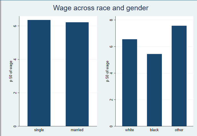
In the title bracket, you can use any title that is required for the graph.
The above generated graph can be saved in hard drive of the computer using the similar command we used above
graph combine g1 g2, saving(combined, replace)