
The collapse command in Stata is used to aggregate a dataset by collapsing it based on some summary statistics of a variable like mean, sum, median, percentile, standard error etc. To understand how a variable can be aggregated, let’s start by loading Stata’s built-in NLSW (1988) dataset.
sysuse nlsw88, clear
We will also drop some variables that are not needed in our example, and then save this new dataset as ‘collapse.dta’.
keep idcode race married wage hours save collapse.dta
Collapsing Data From Stata’s Menu using Collapse Command in Stata
The collapse command in Stata can be used to aggregate the dataset from Stata’s menu options by following:
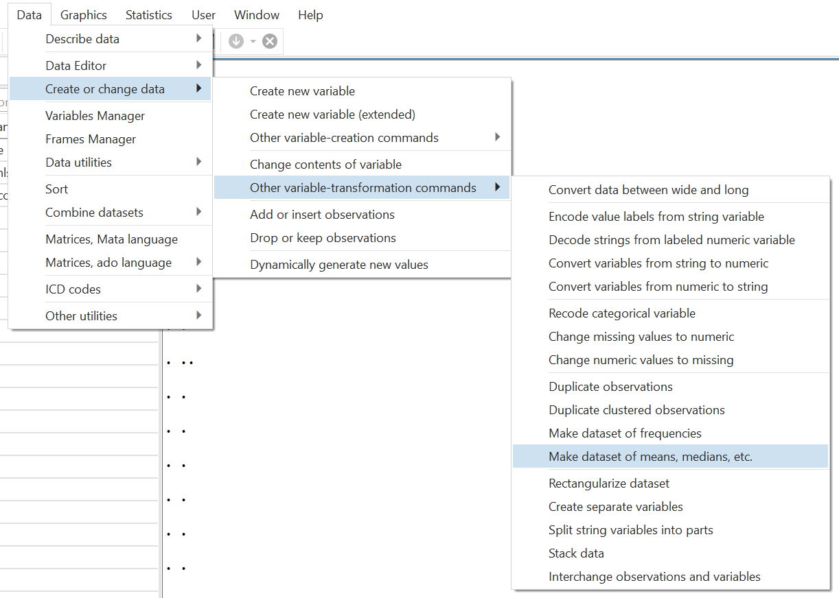
Data > Create or change data > Other variable-transformation commands > Make dataset of means, medians, etc.
In this article, we will focus on the command.
Related Article: Rolling Beta and rolling mean, median in Stata
The collapse Command in Stata – Aggregating Data
A general example using the collapse command in Stata is:
collapse (mean) wage
The statistic name is the bracket refers to how we would like our data to be aggregated, followed by the variable name on which that aggregation is supposed to be based on. In this case, we want our data to be collapsed/aggregated into the mean of the variable ‘wage’.
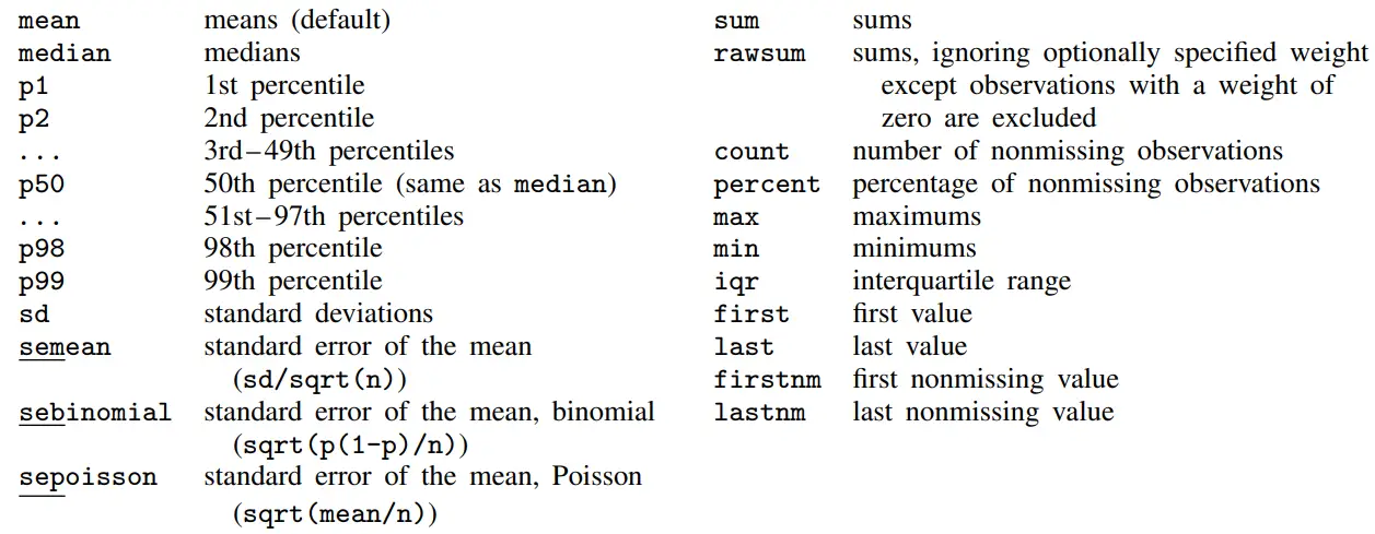
The following is a list of statistics provided in Stata’s help section (help collapse) that can be used with the command.
In the example above, our data would collapse down to just one observation and one variable, which would be the mean of variable ‘wage’.

If you do not specify a statistic in the brackets, Stata will assume it to be the mean by default. Running the command above will be similar to running:
collapse wage
Aggregating/Collapsing Data Based on a Variable and a Category
The example above illustrated the basic function of the collapse command, but perhaps such a simple application will hardly ever be meaningful or useful. In the next example, we will collapse the data on a certain variable’s statistics again. However, this time, it will do so based on the categories of another variable.
Let’s reload the dataset again.
use collapse.dta
We will now aggregate the data by the mean of the variable ‘wage’ categorised by each category of the ‘race’ variable.
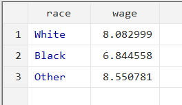
This will collapse the data into the three observations for each category of ‘race’, and two variables: ‘race’, and the mean of ‘wage’.
You can also add multiple categories when using collapse command in Stata to collapse data.
collapse (mean) wage, by(race married)
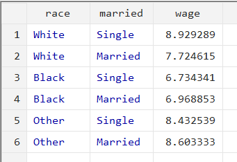
Now, the collapse command aggregates the data into means of the ‘wage’ for each category of the ‘married’ and ‘race’ variables together.
Related Article: Correlation Analysis in Stata (Pearson, Spearman, Listwise, Casewise, Pairwise)
Aggregating/Collapsing Data Based on One Parameter for Multiple Variables
Previously, the mean parameter was only being applied to one variable, ‘wage’. But we can also apply these statistical parameters to more than one variable.
In this example, we want the sum of the number of hours worked and wages earned categorised by ‘race’.
collapse (sum) wage hours, by(race)
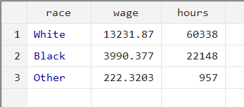
The collapsed variables of ‘wage’ and ‘hours’ are the sum of the wages earned and hours worked by each category of ‘race’. White people worked a total of 60,338 hours and earned a total of 13,231.87 dollars in wages. Meanwhile, black people worked for 22,148 hours in total and earned 3,990.377 dollars in wages. People of ‘Other’ racial backgrounds worked for 957 hours and earned a sum of 222.3203 dollars.
Aggregating/Collapsing Data Based on Multiple Parameters for Multiple Variables
Now, we will see how data can be collapsed based on multiple statistical parameters and multiple variables.
collapse (sum) wage (mean) hours, by(race)
With this command, we want the data collapsed down to the sum of ‘wage’ for each category of race, and the mean of ‘hours’ for each category of race.
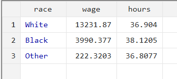
So, the first observation shows that white people earned a total sum of 13,231.87 in wages, with an average number of 36.9 hours worked.
Aggregating/Collapsing Data Based on Multiple Parameters for One Variable
What if you wanted to collapse the data based on, say, both the mean and the sum of one variable? Let’s run the following command:
collapse (sum) hours (mean) hours, by(race)
Here we are asking Stata to aggregate data by the mean and the sum of ‘wage’. The command produces the following error:
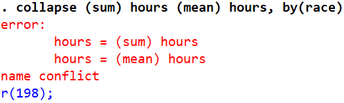
This is because whenever we collapse our data, the variable names stay the same. In our previous examples, we saw that whether we collapsed it by the sum of ‘wage’ or the mean of ‘wage’, the collapsed data still referred to the variable as ‘wage’.
In this case, Stata cannot store the sum of ‘hours’ and the mean of ‘hours’ in the variable called ‘hours’. So it produces an error which tells us that there is a variable name conflict.
To get around this issue, we specify the name of the variable that should be created when storing the sum or the mean (or any other stat) of a variable. This is done by a simple addition to the syntax:
…new_variable_name = existing_variable_name…
Our command above becomes:
collapse (sum) sum_hours = hours (mean) mean_hours = hours, by(race)
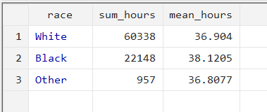
Now, the command collapses the data into the three observations for each category of ‘race’, as well as two new variables for the sum of hours and the mean of hours.
Casewise Deletion When Collapsing Data in Stata
Sometimes, when adding multiple variables to our collapse command, we may find that the number of non-missing observations do not match amongst variables, i.e. some variables may have some missing values while others don’t. What if we only want the collapse/aggregation calculations to be applied to observations that have data for all variables available. As an example, let’s introduce some missing data to our data for ‘wage’.
summ wage hours replace wage=. in 1/500 summ wage hours
Before introducing 500 missing values to the ‘wage’ variable, we summarised ‘wage’ and ‘hours’. We noticed that ‘hours’ had four observations less. After adding the missing values to ‘wage’, it has 1,746 observations and ‘hours’ has 2,242 observations.
Now, let’s collapse/aggregate the data based on the observation count of these variables.
collapse (count) wage hours
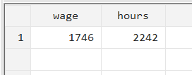
As can be seen, the collapse command in Stata was applied to the available observations for each variable, respectively. No casewise deletion took place. If we were to replace (count) with (mean), the mean for ‘wage’ would be calculated for its 1,746 observations. Similarly, in the case of ‘hours’, for its 2,242 observations.
In order to introduce casewise deletion, we need to add the cw option to the command. This ensures that the (count) or (mean) calculations only use observations where data for both the variables is available.
collapse (count) wage hours, cw
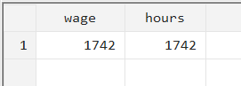
After adding the option, we can see that the output matches for both variables because the command only counted the number of observations where data for both ‘wage’ and ‘hours’ was present.
Related Article: Stata Command Modifiers if, in, by, bysort Qualifiers and Statements in Stata
Adding an if Condition to the collapse Command in Stata
We can also add an if condition when collapsing data so that the statistical calculations are only performed on the subset of data we specify. For example:
collapse (count) wage if wage>30, by(race)
In this case, Stata will collapse the data into the categories of ‘race’, and add an observation count for the ‘wage’ variable only when ‘wage’ is greater than 30.
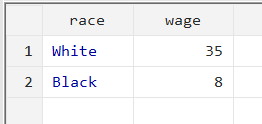
The collapsed data shows that ‘wage’ was greater than 30 for 35 white people, but only for 8 black people.
Using Weighted Average When Aggregating/Collapsing Data
Data can also be aggregated/Collapsed in Stata using the weighted average of a variable.
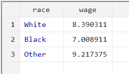
collapse (mean) wage [fw=hours], by(race)
This command will collapse the data into mean of ‘wage’ for each category of race using frequency weights for ‘hours’.
Weighted averages could be helpful with stock market data for various industries, where weighted average stock returns need to be evaluated. The frequency weight in such an example would be the market capitalization of a company, and the by() option would be the industry variable.
How is Weighted Average Calculated?
Let’s end this article with a breakdown of how a weighted average is actually calculated in an example like above.
This is the command we will try to understand:
collapse (mean) wage [fw=hours], by(race)
First, the total number of hours worked for each race category are calculated. Let’s store this in a variable called ‘total’.
bys race: egen total = total(hours)
Then, each individual’s proportion in this total number of hours worked is calculated as a percentage. Remember that because the ‘total’ variable was calculated for each racial category, this proportion will also be the individual’s proportion of hours worked within their own racial category.
gen percentage = hours/total
This proportion is then multiplied with the variable ‘wage’. This is the variable that we actually want weighted based on hours.
gen multiply = percentage*wage
Finally, for each category of race, a sum of this weighted wage is calculated, which is the final value that we are looking for. This value of wage is weighted by the number of hours worked.
bys race: egen wage_avg = total(multiply)
We can check the results either through the browse window or by checking the mean of the ‘wage_avg’ variable for each race.
mean wage_avg, over(race)
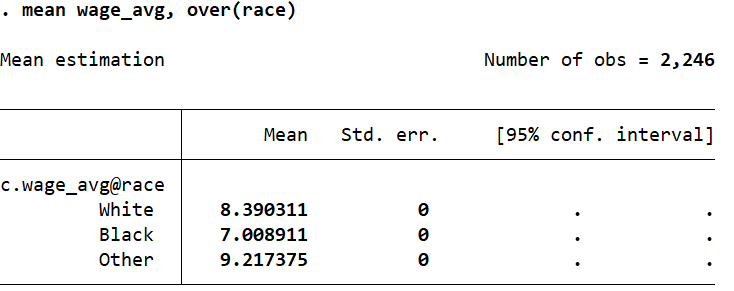
These values match the results we got from the collapse command above.