In Stata, the functionality of commands can be enhanced by adding qualifiers like if and in, and prefixes like by and bysort. Qualifiers are written in the middle of a command to let the command be applied on a specific subset of data. Prefixes are always written at the start of a command and make sure that the command is run for multiple subsets of the data. For example, an if qualifier may be used to run a command on observations for females only. by and bysort may be used to run a command on the entire data but separately for each category (e.g. males, and females).

To explore each of the qualifiers and prefixes further, we will use Stata’s built-in Automobile dataset.

sysuse auto, clear

We will only work with the ‘price’ and ‘rep78’ variables so we will only observe those in the browse window.

br price rep78

You can also check and uncheck the variables that you want to observe from the panel on the right side in the browse window.

The if Qualifier

Related Book: Data Management Using Stata by Michael N. Mitchell

Generating Variables Based on a Condition

We want to generate a dummy variable which will be equal to 1 only if the repair variable, ‘rep78’ is equal to 3. We can use the generate command to create that new variable and add an if qualifier to specify our condition.

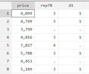
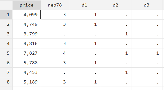
gen d1 = 1 if rep78==3

When you browse the variables ‘price’ ‘rep78’ and ‘d1’, you will note that the new variable ‘d1’ is equal to 1 only when ‘rep78’ is 3. The if qualifier ensured that the generate command was run only when its condition was satisfied. When, for example, ‘rep78’ is equal to 4, the generate command did not assign 1 (or any value) to ‘d1’; it just added a missing value.

The if qualifier can be used with multiple commands. In the example below, we use it to summarize the variables in the dataset only when a car’s price is above 6000.

summ if price>6000

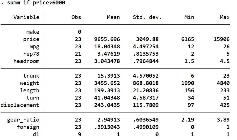
This dataset has 74 observations. However, since we used the if qualifier to restrict the summary statistics to only be displayed for those car that have a price over 6000, this command will return a table with the summary data of only 23 such cars.

Let’s generate another variable using the if qualifier and also explore another issue that you may encounter in Stata.

gen d2 = 1 if rep78>3

When you browse the four variables, you will observe something a little confusing.

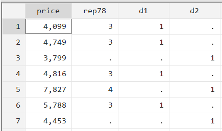
While ‘d2’ does appear to take the value of 1 when ‘rep78’ is greater than 3 (e.g. in the fifth observation), it is also displaying 1 when ‘rep78’ is missing. This is because Stata treats a missing value as the “largest possible value” and will therefore include them when we run commands that have to include values “greater than” a number.

Note that Stata does not treat missing values as a very large number in regressions. When running regressions, it just uses casewise deletion to omit any observation that has a missing value.

This problem can be resolved by adding another condition to our command.

Specifying TwoConditions Using the ‘And’ (&) Operator

gen d3 = 1 if rep78 > 3 & !missing(rep78)

This command will run only if two conditions are met simultaneously: if ‘rep78’ is greater than 3, and if ‘rep78’ does not have a missing value.

The two conditions are added to the command through the and operator which is specified using the ampersand sign, ‘&’. This sign ensures that the command is run only if the conditions written before it and the conditions written after it are fulfilled.

As can be observed in the data, ‘d3’ is no longer equal to 1 when ‘rep78’ has a missing value.

In case you wish to ensure that missing values are ignored for more than one variable, simply add the variable name to the second condition as done below.

gen d4 =1 if rep78>3 & !missing(rep78, price)

The second condition after the and operator will execute the command only for observations where not only is ‘rep78’ greater than 3, but also where ‘price’ and ‘rep78’ do not have any missing values.

Specifying TwoConditions Using the ‘Or’ ( | ) Operator

We can also use the if qualifier and the ‘or’ operator to add conditions where a command is run if any one (or more) of the conditions specified are met. Such ‘or’ conditions are written using the vertical bar, also known as pipe: | . Both the ‘or’ and ‘and’ operators can be used in a single command if need be.

gen d5 = 1 if rep78==3 & (price<4000 | price>10000)

Let’s break down the command above. This command will run for two kinds of observations: where ‘rep78’ is equal to 3 and ‘price’ is less than 4000 or where ‘rep78’ is equal to 3 and ‘price’ is greater than 10000.

Another way to put it is: Stata will check whether a car costs less than 4000 and if ‘rep78’ is equal to 3 or whether a car costs above 10000 and ‘rep78’ is equal to 3. If either of these two conditions are met, variable ‘d5’ will get a value of 1. In any case, ‘rep78’ has to equal 3.

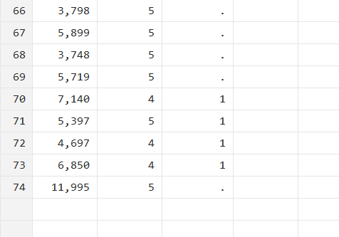
Let’s look at the data from the browse window. But first, we will sort data by ‘price’ so that values less than 4000 are easier to observe.

sort price

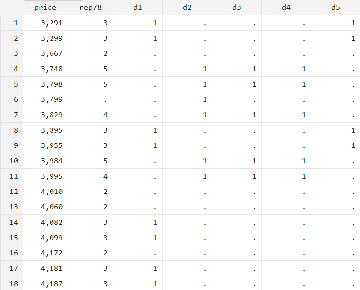
As can be observed, the variable ‘d5’is equal to 1 when price is less than 4000 and when ‘rep78’ is 3 only.

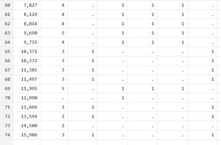
Similarly, as shown in the figure above, ‘d5’ (last column) shows a value of 1 when the price is above 10000 and when ‘rep78’ (second column) is equal to 3.

Whenever we use parentheses ( ) in our commands, Stata uses a rule similar to the one applied in maths i.e. solve the brackets first. In this case, when generating the new variable, Stata first checks whether the conditions in the parentheses are being met or not. In this case, because we include an ‘or’ operator in the parentheses, it checks if the price is less than 4000, or if it is greater than 10000. Once this is done, Stata then proceeds to check the conditions outside i.e. whether ‘rep78’ is equal to 3 or not.

The in Qualifier

The in qualifier in Stata can be used to perform commands on certain rows/observations. For example, we can generate a variable and use the in qualifier to specify which rows/observations that command needs to be applied to.

gen d10 = 1 in 5

The in 5 part of this command simply means that the command is to be executed only for the fifth row/observation in the data.

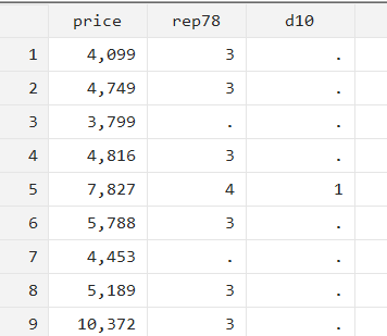
When we run the command, it can be seen that the new variable ‘d10’ is created and takes a value of 1 only for the fifth row/observation.

The in qualifier can also be used to display data from specific observations using the list command.

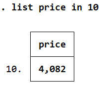
list price in 10

This will output the tenth observation’s price.

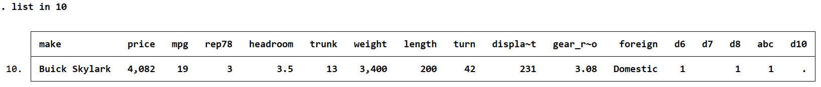
If you don’t specify a variable, it will just output data for all the variables for that particular observation.

list in 10

You can also output data for a range of observations.

list price in 1/10

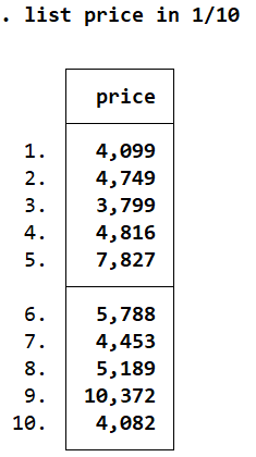
The slash is used to indicate range. Here, 1/10 means rows 1 till 10.

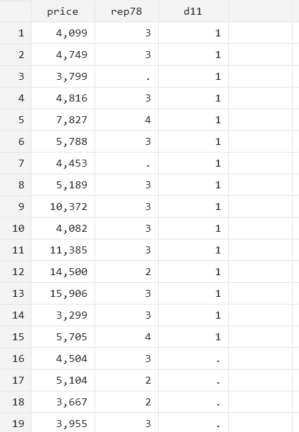
You don’t need to write 1 to refer to the first row, it can also be referred to by writing f.

gen d11=1 in f/15

This generate command will create a new variable called ‘d11’ which will be equal to 1 only from the first observation up until the fifteenth one. All observations after the fifteenth will have a missing value.

You can also use this syntax with other commands like summarize or regression commands. The command will then only be run on the range of observations specified. The following summarize command summarizes price data only for the first 15 observations.

summ price in f/15

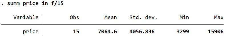
summ price in f/15

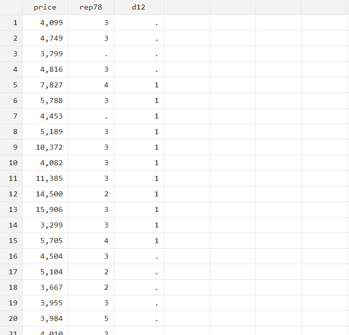
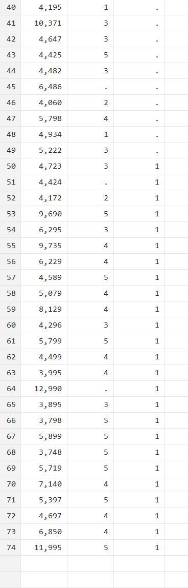
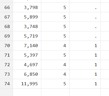
It is also not necessary to always start from the first observation. The following command generates variable ‘d12’ as equal to 1 for rows/observations 5 till 15. Observations 1 till 4 will have a missing value, as will observations 16 onwards.

gen d12=1 in 5/15

You can also refer to the last row/observation by the letter l instead of writing the actual number.

gen d13=1 in 50/l

This command generates a variable ‘d13’ as being equal to 1 for observation number 50 up until the last one.

All observations before row 50 will have a missing value, while the 50th row up until the last one will be 1 for variable ‘d13’.

We can also specify the range of rows/observations in reverse. In the examples above, the range started from a row number, and went forward up till another row number. As such, a range that goes backward can also be written.

gen d14=1 in -5/l

This command refers to the final five observations. Instead of writing numbers to refer to these rows/observations (70/74), we can add a negative sign to the number of observations that are to be counted in reverse from the number after the slash. -5/l means the five observations counted in reverse from the last one.

All observations above the 70th one will have a missing value.

It helps to look at these ranges as Stata counting backwards from the last observation. It also helps to start this counting from the number after the slash. So, -5 would mean five observations counted up from the end of the dataset (i.e. the last five observations).

In the following command, Stata will start from the second observation from the last one (as indicated by -2) and go up till the fifth observation from the last one (as indicated by -5). The observations that fall in this range will get a value of 1.

gen d15=1 in -5/-2

Statements

The if Statement

In the examples above, we looked at the if qualifier. Let’s look at the if statement now.

When writing if statements, we can start by directly typing if followed by the conditions and an opened curly bracket. In the next line, we write the commands that we want executed should the conditions be true. The statement is then closed by a closed curly bracket in the last line.

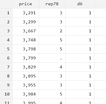
The following if statement attempts to create a variable ‘d6’ which will be equal to 1 if ‘rep78’ is equal to 3.

if rep78==3{
            gen d6 = 1
}

When you browse these variables, you will note that ‘d6’ takes on a value of 1 for all observations regardless of whether ‘rep78’ is 3 or not.

Before getting into why this is happening, let’s try one more command with the if statement.

if rep78==4{
            gen d7 = 1
}

After running this command, you will note that actually no variable called ‘d7’ was generated.

Why is Stata not generating a new variable? And why did Stata assign the value of 1 to all observations despite our if statement?

The if statement in Stata only looks at the first observation when evaluating conditions and executing commands. When we tried to generate the ‘d6’ variable, it checked whether ‘rep78’ had a value of 3 on the first observation. The condition was true, so it proceeded to run the generate command inside the curly brackets.

When we attempted to generate the ‘d7’ variable, the condition of ‘rep78’ being equal to 4 was not met in the first observation, so the generate command inside the curly brackets was not run at all. The if qualifier, on the other hand, evaluated the conditions for each individual observation.

Therefore, when working with variables in Stata, the if qualifier is the better choice rather than the if statement.

In Stata, we should use if statements when we’re working with constant numbers and our command does not depend on some variable. For example, we can use macros with if statements. Among other things, macros are used to store statistics from a summarize command after it is run.

summarize price
return list

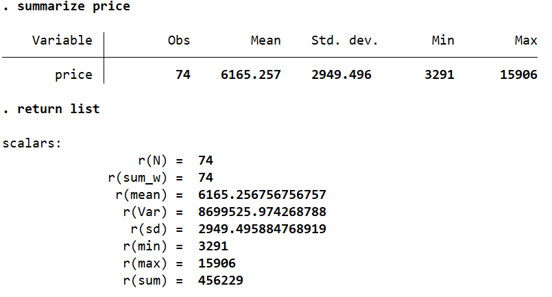
We can use the names of these scalars to refer to the constant values stored in each one. For example, the scalar called r(N) stores the number of observations, and r(mean) stores the average of the variable we summarized.

We can use these with if statements as follows.

summarize price
if `r(N)’==74 {
            gen d8 = 1
}

This is a very simple example, but this statement intends to generate variable ‘d8’ which will take a value of 1 if r(N) i.e. the total number of observations is 74. Remember to run the summarize command before the if statement.

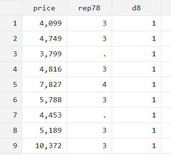
In this case, because r(N) was equal to 74, ‘d8’ is 1 for all observations.

The else Statement

If we want to tell Stata what to do in case the conditions in our if statements are not met, an else statement after our if statement can be added. Let’s change the condition a little by changing r(N)’s value to 75.

summarize price
if `r(N)’==75 {
            gen d9 = 1
}
else {
            gen abc = 1
}

If r(N) is not equal to 75, Stata will not execute the commands in the curly brackets after the if statement, instead, it will move to the else statement and execute the commands written inside its curly brackets.

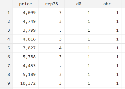
As can be observed, instead of executing the command in the if statement and generating the ‘d9’ variable, Stata moved to the else statement and generated the ‘abc’ variable.

Prefixes in Stata: by vs bysort (Which one should you use?)

by and bysort are prefixes in Stata that can be written before a command. Prefixes are written before a colon at the start of a command. These prefixes help to execute the command on a specified group or categories of observations.

bysort foreign: summ price

In the command above, we are asking Stata to execute the summarize command separately on each of the categories in the ‘foreign’ variable. This variable has two categories, foreign and domestic. Stata will produce summary statistics separately for the foreign cars, and separately for the domestic cars.

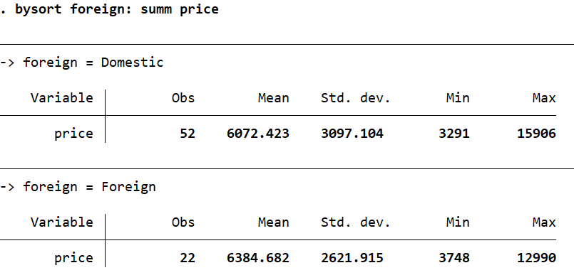
As can be seen from Stata’s output, the 52 observations for domestic cars, and 22 observations for foreign cars were summarized separately. If there were more categories in this variable, say four, Stata would have produced as many summary statistics tables.

When we run the command above with the by prefix, the exact same output is produced.

by foreign: summ price

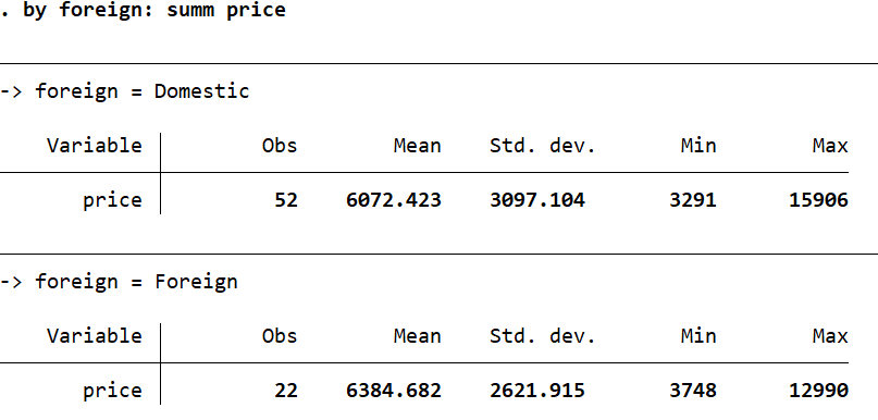
This is because, bysort first sorts the data based on the variable we specify before the colon, and then performs the command. The by prefix does not sort the data.

As can be seen by browsing the data, the data is sorted on the ‘foreign’ variable since we ran the command with the bysort prefix.

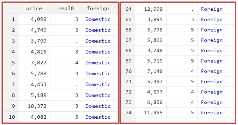
The first 52 observations are for domestic cars, while the last 22 observations correspond to foreign cars.

Let’s sort the data on some other variable and rerun the summarize command with the by prefix.

sort price
by foreign: summ price

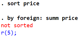
Stata can no longer run the command because the data is not sorted by the categories that we are asking it to summarize the data for.

While this may make it seem like the by prefix isn’t very useful, that is not the case. Remember that the bysort prefix sorts the data every single time it is run, even if the data is already sorted for the categorical variables specified. When we are working with very large datasets, it becomes too time consuming for the data to be sorted each time a command is run. For such datasets, it is more efficient to sort the data just once, and then use the by prefix to run any commands that we need to execute on the different categories of that sorted variable.

sort foreign
by foreign: summ price

Sorting the data on ‘foreign’ would allow the summarize command with the by prefix to run smoothly.

Once the data is sorted on ‘foreign’, we can run as many commands with the by foreign: prefix as we want without compromising on the efficiency of our code.

sort foreign
by foreign: summ price
by foreign: summ mpg
by foreign: reg price rep78

Finally, data can still be sorted while using the by prefix by adding an option of sort to this prefix.

by foreign, sort: summ price

This command works exactly like the one with the bysort foreign: prefix.

Stata Command Modifiers if, in, by, bysort Qualifiers and Statements in Stata