
This article will help you to estimate the beta (weekly, monthly, and annually) using STATA. The focus will be on the command statsby.
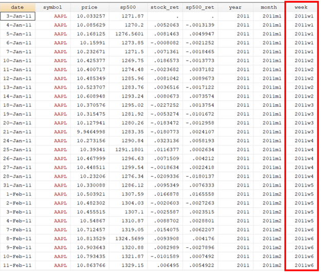
The provided dataset has four variables (date, symbol, price, and S&P 500). The data comprise four firms (AAPL, GE, GM, and MSFT)
To calculate the beta, it is a must to calculate the four firms stocks return and market return. For this, we will use the below commands:
Download Example Filebys symbol (date): generate stock_ret = ln(price / price[_n-1]) bys symbol (date): generate sp500_ret = ln(sp500 / sp500[_n-1])
We will begin the command bys, write the variable name representing firms (symbol), and sort the data based on the variable date. The bysort will repeat the command for each firm separately hence we are telling Stata that there are different firms (symbols). The date in parenthesis tells Stata to first sort each firm’s data by date and then perform whatever command comes after colon “:”. Then, we will write the name of the new variable we want to generate. The new variable will be created by dividing the natural log of the current year’s stock price by the previous year’s stock price.
To estimate the beta, following command will be executed:
statsby , by(symbol) saving(firm_beta,replace): regress stock_ret sp500_ret
There are multiple firms in our dataset; therefore, the regression will be repeated for all the firms separately. To do so, the by option has been used after the command statsby. The option saving has been used to save the beta generated as statsby saves betas into a new data (.dta) file . Replace option has also been used with the saving option so that any file saved with the same name is replaced with a new file. Lastly, the regression command has been used to regress stock return on market return (S&P500). When we execute this command, the new file will generate with the name file_beta.
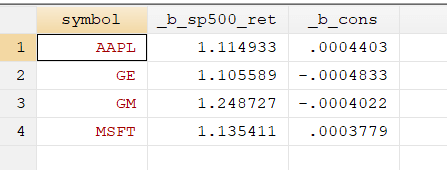
The screenshot of the firm_beta file is presented below:
Related Book: Introductory Econometrics for Finance by Chris Brooks
The statsby command can also be accessed following the below path:
Statistics > Other > Collect statistics for a command across a by list
If instead of generating a new file with betas, we want all the betas to be generated in the current file then we can use clear option instead of saving option. clear option will clear all the data in current memory and bring the generated betas in the memory.
statsby , by(symbol) clear: regress stock_ret sp500_ret
There is also an option of providing a name to the beta and constant variable generated using the statsby command. The below command will be used for that purpose:
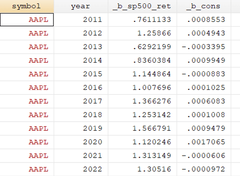
statsby beta=_b[sp500_ret] cons=_b[_cons] , by(symbol) saving(firm_beta,replace): regress stock_ret sp500_ret
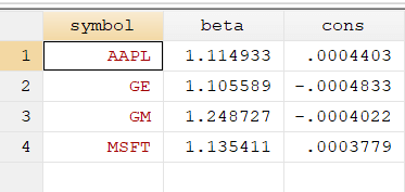
After the statsby command, the name of the new variable (beta), then after “=” the calculation we want to perform and save. Similarly, the name of the second new variable (cons). The rest of the command will remain the same. After executing the command, we will get new variables named beta (previously b_sp500_ret) and cons (previously _b_cons).
Related Article: Rolling Beta and rolling mean, median in Stata
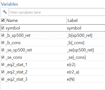
Along with the betas and constant values, we can also calculate the standard errors, r2 and adjusted r2, and the number of observations using the below commands.
statsby _b _se e(r2) e(r2_a) e(N), by(symbol) saving(firm_beta,replace): regress stock_ret sp500_ret
_se e(r2) e(r2_a) and e(N), are representing standard error, r2 , adjusted r2 and number of observations. The rest of the command will remain the same.
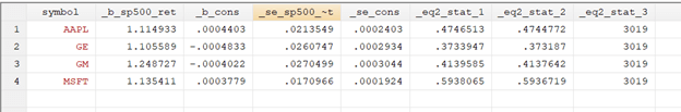
The additional variables will be generated in the firm_beta file, as shown in the above figure.
All the above commands have generated a single beta for each firm by taking all the data into account. However, if we want weekly, monthly, and annual beta, the commands require some changes.
Yearly Beta
The first step will be extracting the year from the date. For that, the below command will be used:
generate year=year(date)
Related Article: Using Dates in Stata | Quick Tips to work with Dates in Stata
By executing this command, you will notice that a new variable (year) will be generated. This variable will represent the years extracted from the date. Then to compute the betas, we will again execute the statsby command. The only change will be adding the year variable with the symbol variable in the by option. Also, _b is added after the statsby command, but it is not necessary to write the _b after the statsby command as by default it would generate the betas.
statsby _b , by(symbol year) saving(firm_year_beta,replace): regress stock_ret sp500_ret
The yearly beta will be computed in a new file named firm_year_beta. For every four firms, the twelve betas will be computed, one for each year.
Monthly Beta
Similarly, to compute monthly beta, we will extract the months from the date variables using the below command.
gen month=mofd(date)
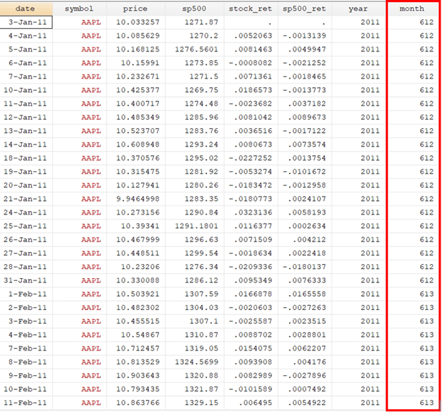
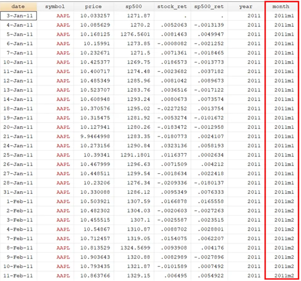
When we execute this command, the variable month will be generated. The STATA will assign a unique value to the months of all four firms. These numbers are not human-readable. To have a better understanding, the month variable will be formatted using the below command:
format month %tm
The data for the month after formatting will look like this:
To compute the monthly beta, the below command will be used:
statsby _b , by(symbol month) saving(firm_month_beta,replace): regress stock_ret sp500_ret
The monthly beta will be computed in a new file named firm_month_beta.
Weekly Beta
Again, to compute the weekly beta, we will extract the week from the date variables using the below command.
gen week=wofd(date)
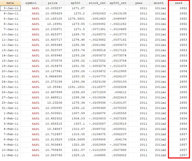
When we execute this command, the variable week will be generated. The STATA will assign a unique value to a week of all four firms. The values are not human-readable. To have a better understanding, the week variable will be formatted using the below command:
format week %tw
To compute the weekly beta, the below command will be used:
statsby _b , by(symbol week) saving(firm_week_beta,replace): regress stock_ret sp500_ret
The weekly beta will be computed in a new file named firm_week_beta.
Related Article: Estimate Rolling Regression or Rolling Beta in Stata
Descriptive Statistics
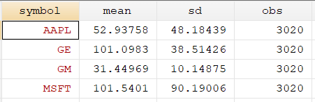
Using the command below, we can also compute the descriptive statistics (mean, standard deviation, and number of observations).
statsby mean=r(mean) sd=r(sd) obs=r(N), by(symbol) clear: summarize price
On executing the above command, the following variables will be generated:
To generate this variable in a new file, use the below command:
statsby mean=r(mean) sd=r(sd) obs=r(N), by(symbol) saving(firm_summarize,replace): summarize price