In field of finance and econometrics, we need to measure the movement of assets according to market movement or Market Beta. Nothing in finance remain constant over time. Cost, finances, and revenues changes from time to time, so we have to move towards the method of moving averages and many like these. So, method of rolling window/regression were defined to observe market beta and how it is changing time to time.
In rolling regression, we take the certain number of observations called estimation window (let’s say 30 days in this case) and we keep on rolling the window till we reach the end of the data. Following example would explain the idea of rolling regression:
1st: Calculate a regression beta for observation from 1 to 30 (Beta for the 30th observation)
2nd: 2-31 observations (Beta for the 31th observation)
3rd: 3-32 observations (Beta for the 32th observation)
And so on.
Let’s calculate this rolling regression using Stata. In this article we will calculate rolling regression using two different commands.
Firstly, we will use rolling command which is built in command, then we will use asreg command which is a user written command. Both of these commands would produce similar results, the only difference is that asreg is quite faster compared to rolling command.
Related Book: Introductory Econometrics for Finance by Chris Brooks
Calculating Rolling Beta using Built-in Rolling command in Stata
Let us take an example of daily stock prices of four different companies i.e. Apple, Microsoft, General Electric and General motors. We also have data of S&P500 index representing the market index.:
Download Example FileWe can open our file using command
use "example.dta", clear
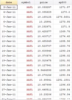
Our dataset contains daily data ranging from 3-Jan-22 till 30-dec-2022.
Now we have to tell Stata that we have a panel data in order to implement the rolling command.
encode symbol, gen(symbol_code) xtset symbol_code date
Firstly, encode command will assign or encode each symbol variable a number because symbol variable is string variable having characters which is not acceptable by xtset command. Xtset require that the variable be in numerical form. Hence, using encode command we have converted symbol (which is a string variable) into a symbol_code (which is a numerical variable) which will have encoded number as:
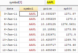

xtset command is used when we deal with panel data, so we have panel data because we have multiple firms and multiple time periods.
We currently have stock prices and S&P500 index in our dataset. However, beta is a linear regression of stock return on market return. Hence, we first need to calculate stock return and market return. The following commands will calculate stock and market return.
bys symbol (date): generate stock_ret = ln(price / price[_n-1]) bys symbol (date): generate sp500_ret = ln(sp500 / sp500[_n-1])
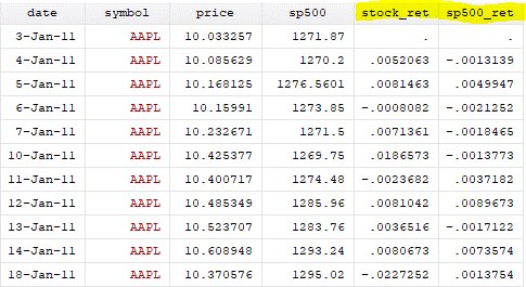
Now we calculate beta using rolling command whole code in Stata as
rolling , window(30) saving(rolling_command,replace): regress stock_ret sp500_ret
rolling is built-in command which will calculate regression of stock_ret on sp500_ret. We start with the command name i.e. rolling and after comma we include a bunch of options. Firstly, we need to tell Stata what will be rolling window. In our example we are estimating regression on 30 days rolling window, hence we use the option window (30). Next, we use the saving option, which tell Stata the file name in which Stata will store the betas. Lastly, following the colon ‘:’, we will use an estimation command, which in this case is the regress (regression of stock return on market return)
Related Article: Rolling Beta and rolling mean, median in Stata
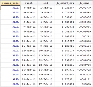
Have output in new file as:
And in this file we have beta values as:
You can use the following full code to execute whole Rolling regression code:
use "example.dta", clear bys symbol (date): generate stock_ret = ln(price / price[_n-1]) bys symbol (date): generate sp500_ret = ln(sp500 / sp500[_n-1]) encode symbol, gen(symbol_code) xtset symbol_code date rolling , window(30) saving(rolling_command,replace): regress stock_ret sp500_ret
Calculating Rolling Beta using Asreg command in Stata
asreg is user written command and if you do not have asreg already installed in Stata you can install it by typing this command in command window of Stata:
ssc install asreg , replace
You can use asreg command to calculate rolling regression in Stata. It is less time taking than rolling command.
We will import a fresh copy of the data and generate the stock return and market return as we did before using the following commands.
use "example.dta", clear bys symbol (date): generate stock_ret = ln(price / price[_n-1]) bys symbol (date): generate sp500_ret = ln(sp500 / sp500[_n-1]) encode symbol, gen(symbol_code) xtset symbol_code date
Lastly, we will execute asreg command as given below:
Related Article: How to Estimate Weekly, Monthly, Yearly Betas in Stata
bys symbol: asreg stock_ret sp500_ret, wind(date 30)
Because we have panel data, so we would execute the asreg command for each symbol separately. Therefore, we are using bys symbol prefix, which would tell Stata to run asreg command for each symbol separately. Lastly, we have wind option, where we provide the name of time variable which in our case is ‘date’ followed by the window size.
This will also calculate data for market beta in Stata as:
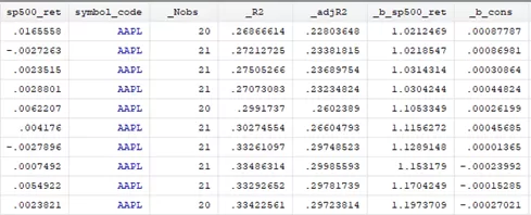
You can compare these results with the results of rolling regression command and realize that both commands produce same results.
Calculating Rolling Regression using Asreg w.r.t Trading Days in Stata
As you can see in above results, asreg command do not take 30 days (check column naming _Nobs in above picture) for calculating beta but 20,21 or 22 days only. We can check it from help of Asreg command in Stata as:
help asreg
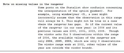
As explained above it will not account for missing days. These are what we call calendar dates, but instead of calendar days, we can also use trading days. We need to generate a trading day variable which is equal to the serial number and by symbol to repeat separately for all four different symbol values to avoid overlapping. We can use the following command in Stata:
bys symbol: gen id=_n
Related Article: Use of System Variables, difference between _n and _N in Stata
Now by running asreg command again in Stata but this time not the date but on trading day (id variable that we just generated) variable which is given above as id:
bys symbol: asreg stock_ret sp500_ret, wind(id 30)
Now the results would be having the values of beta for entire 30 days from row 31 onwards:
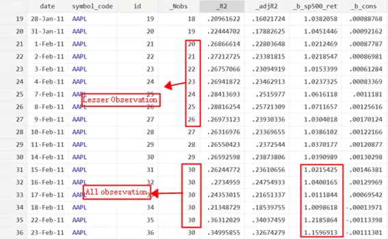
As you can see it took full 30 days atleast from the row 31st onwards as marked with “All observations”. For ID value less than 30 in above figure you can see there are lesser observations as this is a short coming in asreg command i.e. it would estimate regression even if number of observations are less than specified in window. We can resolve this by either dropping any rows that have less than 30 observations or use min option in asreg as explained below.
Setting Minimum Value of observation for Rolling Regression using asreg command in Stata
Setting minimum value during asreg command can help us removing extra useless values that we do not need because our window for beta is 30 observation.
We can use min option in asreg to set for minimum value as follows:
bys symbol: asreg stock_ret sp500_ret, wind(id 30) min(30)
Results are as:
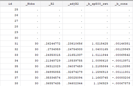
As you can see now all the beta values that were before are no more now. It is starting from where it has all 30 observations to calculate for regression value.
Window option while using Asreg Command in Stata
There are multiple ways to use window (wind) option:
window(rangevar #from #upto)
The syntax of window option looks like as shown above. We need to specify the rangevar (i.e. the date variable) then the range #from and #upto values. rangevar and #from is mandatory, #upto by default is zero.
Backward Looking Window
Related Article: Estudy Command for Event Study in Stata
In backward looking, window option will take all the values in the backwards and calculate beta for like for example:
window(id -30 0)
It will take all values from 1 to 30 to calculate for beta value corresponds to observation 31. For Stata we have command:
bys symbol: asreg stock_ret sp500_ret, wind(id -30 0) min(30)
Results are pretty much the same as we have implemented asreg with 30 only.
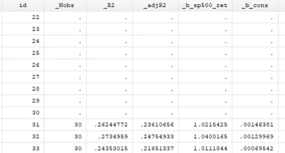
But if we take -10 instead of 0 it will take only 1-20 observation for calculating beta corresponds to observation no 31.
bys symbol: asreg stock_ret sp500_ret, wind(id -30 -10)
As a result:
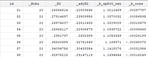
It took only 20 observations although for trading days variable but -10 will decrease 10 recent observations while calculating beta.
Forward Looking Window
In forward looking, number from is less than the number upto means if I want to calculate value for 30 and make second variable as 50, it will take next 20 observation to calculate beta for regression value.
This also explained good in help manual too.
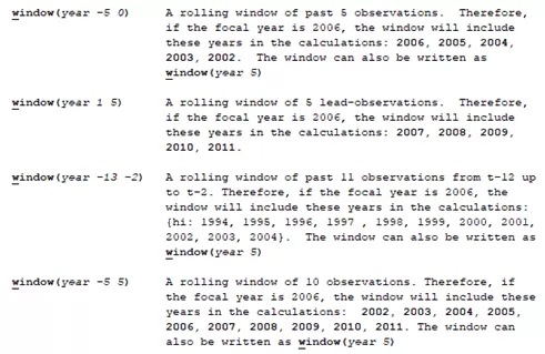
Fitted and Residual values while using Asreg Command in Stata
Fitted and residual values can also be found while calculating beta by using fitted option in the end. Fitted values are the values that are predicted from all previous observations, and residual values are difference between observation and fitted value.
By using command as following in Stata, we can calculate residual as well as fitted values while calculating beta:
bys symbol: asreg stock_ret sp500_ret, wind(id 30) min(30) fitted
You will get fitted and residual values as:

Recursive window while using Asreg Command in Stata
Recursive means repeating. As in asreg command we are calculating regression and beta value, if we want to consider all observations again and again to see impact on the beta value then we use this recursive option. We can use recursive option to include recurring observations as by using the command:
bys symbol: asreg stock_ret sp500_ret, wind(id 30) min(30) recursive
We have the result as:
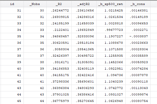
As you can see first it took the first 30 observations and calculated beta, then it took all previous 30 and a plus new 31st observation and calculated beta for 32nd observations. And as the calculation continues you will see starting point of data is same for every observation and ending point is varying as observations are moving down.
Excluding observation, while using Asreg Command in Stata
If we want to exclude any observation while calculating the beta we can use exclude option. Sometimes we come up with data that have some observations that are not matching other data we can exclude it from calculating beta. For example, I want to exclude the current observation on which we are working for beta we can use exclude option as:
bys symbol: asreg stock_ret sp500_ret, wind(id 30) exclude(id 0 0)
We have the result as:
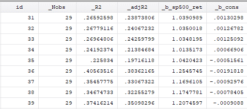
As we can see from above results it started taking only 29 observations instead of 30. So, for thirty-one observation it excluded the 30th one and calculated for regression value.
There are other options that you can explore as well such as noconstant, se (standard error), newey(2), robust etc.
Difference between rolling and asreg
The only difference between rolling and asreg is that of speed, the latter is faster. To compare the speed of these two commands we are going to switch on rmsg. Now whatever command we execute we will get the execution time of the command
Set rmsg on
We are going to execute the same rolling and asreg commands that we did previously, this time just to measure the execution time.
rolling , window(30) saving(rolling_command,replace): regress stock_ret sp500_ret

bys symbol: asreg stock_ret sp500_ret, wind(date 30)

It took rolling command 455 seconds (7.5 mins) to perform same analysis as done by asreg in 45 seconds. So if you have more time at your hand, use rolling 😊 .
You can switch off rmsg:
set rmsg off
