Estudy Command for Event Study in Stata

In the previous article, we studied the event study basics. It was discussed that finance and economics; event studies are frequently used to examine the influences of corporate events on the stock prices of affected companies, and it implements in five steps that include, identifying the event of interest, deciding the estimation window, deciding the event window, calculating the Cumulative Abnormal Return (CAR)  or Buy-and-hold abnormal return (BHAR) and testing the significance of AR and Cumulative Abnormal Return (CAR). In this article, we will perform all these steps using STATA. Download the data and do file from the link given below:

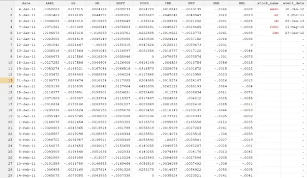
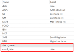
Download Code and Data

The dataset we are going to use to conduct the event study comprises the following variables:

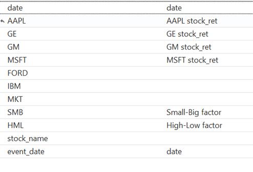
The variables included are the return for different stocks and market return.  It also consists of the data for the  SMB and HML factors, along with the dates of events. The SMB is the return spread of the small minus large stocks. The tendency of smaller firms to outperform their larger counterparts over time is captured by this factor. It is quantified by comparing the returns on small-cap stock and large-cap stock portfolios. HML is the return spread of the high and low prices stocks. The factor account for the tedency of the firms with a lower price-to-book ratio tend to outperform those with a high price to book ratio.

The initial step is to install the estudy command using the below command.

ssc install estudy

To conduct the event study analysis in Stata, we need to have data in a wide format.

 Note: If the data is not in wide format, convert it into wide format before proceeding further using “reshape” command.  The command that will calculate the Cumulative Abnormal Return (CAR) or Cumulative Average Abnormal Return (CAAR) and also conduct the t-test for the event study is given below:

estudy AAPL GE,datevar(date) evdate(01072011) dateformat(DMY) lb1(0) ub1(3) eswlb(-120) eswub(-10)  indexlist(MKT)

First of all, we will write the command estudy and then the name of the companies on which we are interested in conducting the event study.  After the comma, we will write the option datevar, and in parenthesis, we will write the time variable that is the date in our dataset.  Then we will write the event date within the parenthesis of the option evdate.  The next option of dateformate will be used to specify the event date format written within the option of evdate.DMY represents the date, month and year.The lb1 (lower boundary limit) and ubl (upper boundary limit) options will be used to set the event window.  In our example, the event window will start on the event date and end three days after the event.

After the event window, we will add the eswlb (lower boundary) and eswub (upper boundary) options to set the estimation window.  We are using a 120-day estimation window that will start 10 days before the event and last 120 days before the event.  During this time period, we will calculate the expected return.  Lastly, we will add an indexlist optionto specify the model we are willing to use.  In Stata, indexlist option will specify the list of variables that we want to add in the regression model. For instance, if we want to use the market model then we will only add “MKT” within the indexlist option.

Related Article: Event Study using the Eventstudy2 command in Stata

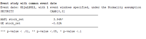
After running the command, we will get the below results:

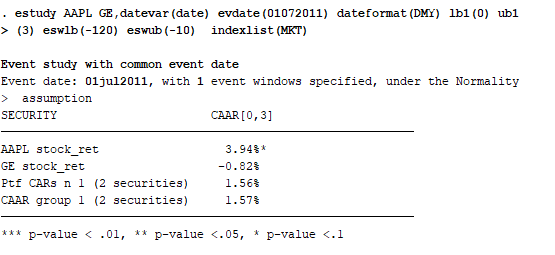
The above results indicate that our event date is July 1, 2011, and there was only one event window.  The event window can be multiple, which will be explained as the article proceeds.  According to the finding presented in the above table, there is a 3.94% increase in the stock return of Apple, which is significant at a 10% significance level.  Whereas the event had a negative impact on General Motors stock return, the results are not statistically significant.  Ptf Cumulative Abnormal Return (CAR) represents the buy-and-hold return.  Lastly,Cumulative Average Abnormal Return (CAAR) is the average Cumulative Average Return (CAR) of Apple and General Motors.

Errors in Event Study

There are multiple errors that can occur in the event study.  The first possible error is that the data is not sorted.  In that case, we will get the below error:

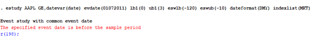
Therefore, it is a must that data be sorted based on date.  The below command is used to sort the data based on date.

sort date

Portfolio or Group

  We can also evaluate the Cumulative Abnormal Return (CAR)  of the multiple portfolios.  To do so, we will run the below command:

estudy AAPL GE (GM MSFT FORD IBM) (AAPL IBM GM),datevar(date) evdate(01072011) lb1(0) ub1(3) eswlb(-120) eswub(-10) dateformat(DMY) indexlist(MKT)

The command will remain the same, but the two more portfolios will be added before the datevar() option within the parentheses.  The parenthese will separate or differentiate the portfolios except for the first one.  The same company can be used multiple times to construct the portfolio.

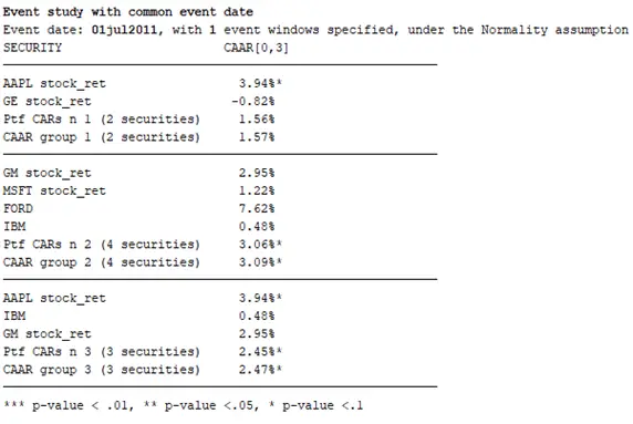
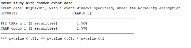
As shown above, we will get the Cumulative Abnormal Return (CAR)  and Cumulative Average Abnormal Return (CAAR) of three different portfolios or groups. The Cumulative Abnormal Return (CAR)  of the inidividual stocks will remain same while the Cumulative Abnormal Return (CAR) of the portfolio will change.

Related Article: How to Create and use Business Calender in Stata

Multiple Event Window

As discussed earlier, We can also use multiple event windows.  These event windows can be more than 1.

estudy AAPL GE,datevar(date) evdate(01072011) lb1(0) ub1(3) lb2(-2) ub2(0) lb3(1) ub3(5) eswlb(-120) eswub(-10) dateformat(DMY) indexlist(MKT)

The command will remain the same; only the additional event windows will be added using lb2, ub2, lb3, and ub3.  The three event windows are (0,3), (-2,0), and (1,5).  On running the above command, we will get the below results.

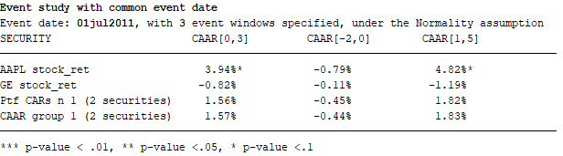
The above result in the table represents the Cumulative Abnormal Return (CAR)  for three event windows.

Model Type:

We can use a different model to calculate the expected returns, such as:

1. Mean Adjusted Return
2. Market Adjusted Return
3. Market Model
4. CAPM
5. FF3 Factor Model

The two things that vary from model to model are the following:

1. modtype
2. indexlist

By default, the Stata uses modtype(SIM)

1. Single Index Model

In a single index model, we can only use one variable in the indexlist option.  CAPM and Market Model have only one independent factor; that’s why they are known as the single index model.  In other words, a single index model means that we will only have one independent variable in our model.  As discussed, the command will remain the same only indexlist, and the modtype will vary from model to model.

estudy AAPL GE,datevar(date) evdate(01072011) lb1(0) ub1(3) eswlb(-120) eswub(-10) dateformat(DMY) indexlist(MKT) modtype(SIM)

In the above command, the indexlist consists of only one independent factor/variable MKT, and the modtype is SIM.  It is optional to write the modtype in this type of model.  So, the below command can also be used without the modtype option.

estudy AAPL GE,datevar(date) evdate(01072011) lb1(0) ub1(3) eswlb(-120) eswub(-10) dateformat(DMY) indexlist(MKT)

2. Market-Adjusted Model

In the market-adjusted model, the market’s return on a specific date will be used as the expected return. The modtype “MAM” will be used for this format.  It must specify this mode type; otherwise, Stata will use the default model type “SIM.”

estudy AAPL GE,datevar(date) evdate(01072011) lb1(0) ub1(3) eswlb(-120) eswub(-10) dateformat(DMY) indexlist(MKT) modtype(MAM)

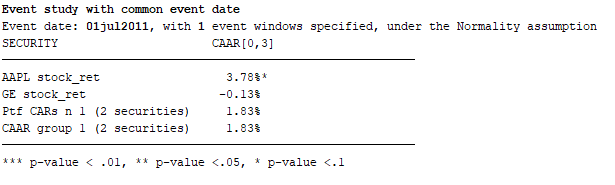
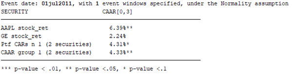
The results obtained through the market-adjusted model are shown below:

3. Multiple Factor Model

Fama French Model is a type of multiple-factor model because it comprises three factors (market, size, and value).  The command for the multiple-factor model is given below:

estudy AAPL GE,datevar(date) evdate(01072011) lb1(0) ub1(3) eswlb(-120) eswub(-10) dateformat(DMY) indexlist(MKT SMB HML) modtype(MFM)

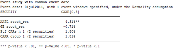
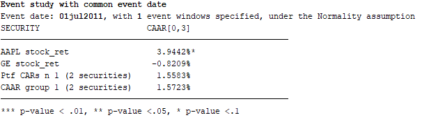
The modtype in the case of a multiple-factor model is “MFM,” The indexlist also comprises three factors or variables: MKT, SMB, and HML.  The results of this model are given below.

4. Historical Mean Model

The last model is the historical mean model, also known as the mean-adjusted model.  In this model, the expected return equals the average return of the estimation window.  This type of model does not have the option indexlist.  Modtype will be HMM, as shown in the below command:

estudy AAPL GE,datevar(date) evdate(01072011) lb1(0) ub1(3) eswlb(-120) eswub(-10) dateformat(DMY) modtype(HMM)

Diagnostic Test:

The Stata uses the t-test by default to investigate whether the difference is significant.  Some other tests can also use, such as Wilcoxon.  The command for this test is given below:

estudy AAPL GE,datevar(date) evdate(01072011) lb1(0) ub1(3) eswlb(-120) eswub(-10) dateformat(DMY) indexlist(MKT) diagn(Wilcoxon)

The diagn option has been added at the end of the command.  Several tests can be used.  The list is given below:

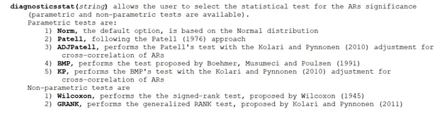
Only one diagnostic test can be run at a time.  Therefore, to use multiple diagnostics tests, the command must be run separately for every type of diagnostic test.

Limiting the Decimal Points

You might notice that we get the results in two decimal places.  To increase the decimals, the dec() option will be added at the end of the command and specify the decimal places as shown below:

estudy AAPL GE,datevar(date) evdate(01072011) lb1(0) ub1(3) eswlb(-120) eswub(-10) dateformat(DMY) indexlist(MKT) dec(4)

You will notice that decimal places increased to 4.

Price

Instead of having stock or market return data, we can have price data.  In that case, we need to specify the price at the end of the command.  It will tell the Stata that we have price data for the different stocks and markets instead of returns.  Stata will calculate the returns itself.  The command is given below:

 estudy AAPL GE,datevar(date) evdate(01072011) lb1(0) ub1(3) eswlb(-120) eswub(-10) dateformat(DMY) indexlist(MKT) dec(4) price

Showpw

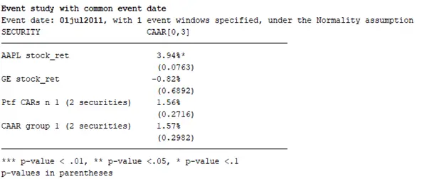
The option of showpv is used to see the p values along with the Cumulative Abnormal Return (CAR).  The below command will be used for this purpose:

estudy AAPL GE,datevar(date) evdate(01072011) lb1(0) ub1(3) eswlb(-120) eswub(-10) dateformat(DMY) indexlist(MKT) showpv

The result of the above command is presented below:

Nostar

Related Book: Introductory Econometrics for Finance by Chris Brooks

We also have a nostar option that helps remove the * with the Cumulative Abnormal Return (CAR)  value.

Storing Results in Excel or dta format

To save the results in excel or dta format, the below commands will be used:

estudy AAPL GE,datevar(date) evdate(01072011) lb1(0) ub1(3) eswlb(-120) eswub(-10) dateformat(DMY) indexlist(MKT) outputfile(excelresults)

estudy AAPL GE,datevar(date) evdate(01072011) lb1(0) ub1(3) eswlb(-120) eswub(-10) dateformat(DMY) indexlist(MKT) mydataset(stataformat)

The results will be exported to the working directories using the above commands.

Suppress

There is also an option to suppress the results.  The first command below will suppress the individual results, while the second command will suppress the group results.

estudy AAPL GE,datevar(date) evdate(01072011) lb1(0) ub1(3) eswlb(-120) eswub(-10) dateformat(DMY) indexlist(MKT) suppress(ind)

estudy AAPL GE,datevar(date) evdate(01072011) lb1(0) ub1(3) eswlb(-120) eswub(-10) dateformat(DMY) indexlist(MKT) suppress(group)

Graphs:

We can also make the graphs by using the below command:

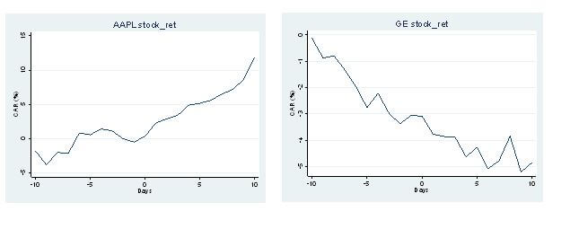
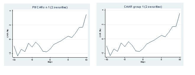
estudy AAPL GE,datevar(date) evdate(01072011) lb1(0) ub1(3) eswlb(-120) eswub(-10) dateformat(DMY) indexlist(MKT) graph(-10 10)

The graph option must be added at the end of the command.  By running this command, four graphs will be constructed.

Different dates for different stock

We can use different dates for different stocks also.  Here, we will use these two variables.

The below command will be used for this purpose:

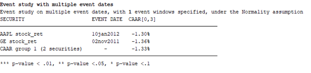
estudy AAPL GE,datevar(date) evdate(stock_name event_date) lb1(0) ub1(3) eswlb(-120) eswub(-10) dateformat(DMY) indexlist(MKT)

Rather than writing the event date, we will specify the stock name and event date variable within the parenthesis of option evdate.  The results are shown below:

Limitation of estudy:

The command estudy does not capture the effect of two events of the same stock.  Such as, if Apple announced the stock split twice into two different dates, then it is impossible to measure the influence of these two events on the same stock using estudy.