How to Reshape Data from Long to Wide form in Stata

This article will go over, in detail, about the reshape command in Stata. This article is motivated by Chapter 9 Data Management Using Stata by Michael N. Mitchell. of It is worth starting by looking at why exactly we need to use this command. The first thing we need to understand before diving into reshape is the concept of “wide form” and “long form”.

Download Example File

The Difference Between Wide and Long Form Data

A dataset is said to be in wide form when data in the first column is not repeated i.e. the first variable is a unique identifier. If the first variable is, for example, student name, it will appear only once in the data. On the other hand, a long form data is one where the first column can repeat multiple times. Whether the data is long form or wide form depends on how it is structured i.e. how many, and what kind of variables are present in it. For example, in some datasets, there is a separate observation for every time period (long form), while in others, there are separate variables for a time unit. Apart from time, there can also be some other subcategory of the first column variable that determines how the data is structured. 

Take a look at these tables that come up when you get help for the command in Stata (help reshape):

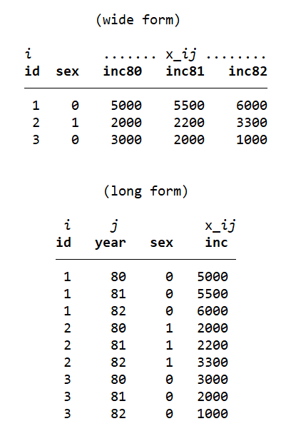
The data displays incomes for three years. In the first, wide form table, a person’s id (‘id’) appears only once. Values for their income for each year are stored in a separate variable for each year (‘inc80‘, ’inc81’, ’inc82’). This way, the year is indicated by the variable name, while the income for that year is stored as an observation. Thus, each year’s income can be stored in a single observation. On the other hand, in the long form example under it, we notice that there is only one variable for year (‘year’), and one variable for income (‘inc’). Thus, each observation shows income data for one single year only. This in turn means that each ‘id’ is repeated three times (has three observations) for each respective year.

Oftentimes, it is hard to conduct appropriate analysis on data if its structure is not in the right format. In such cases, the reshape command comes in handy. We will now go over various examples where there’s a need to reshape the data into one form or the other. These examples include reshaping for single and multiple variables, numeric variable names, string variable names, special characters in variable names, and multiple unique identifiers.

Loading Our Dataset

We will use a pre-existing dataset for our reshape exercise in this example. It can be loaded into Stata through the command:

webuse reshape1, clear

Reshaping For Single Variable

You will note that this dataset has two cross-sectional variables (‘id’ and ‘sex’), and six time variables. ‘inc80’, ‘inc81’ and ‘inc82’ store income values for each of the years indicated by the suffixes, while ‘ue80’ ‘ue81’ and ‘ue82’ are three variables storing unemployment data for the years indicated by the suffixes. Clearly, this is a wide form dataset. Reshaping it to long would create one variable for year, and one variable each for any other metric that has yearly observations.

Since this example focuses on reshaping for a single variable, let’s drop the unemployment variables.

drop ue*

(The asterisk indicates that all variables with the prefix ‘ue’ be dropped).

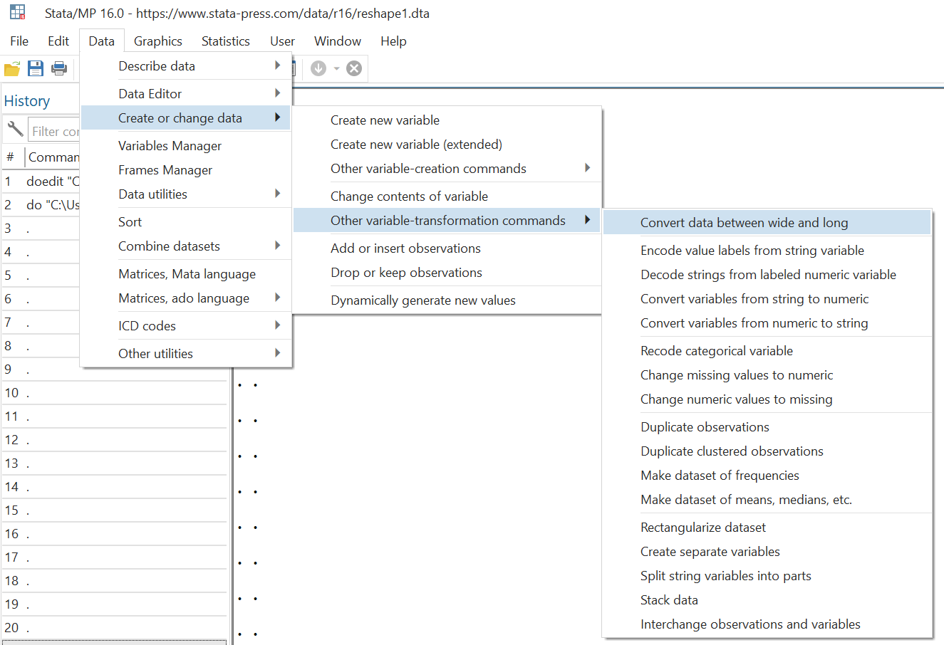
Before diving into the reshape command, let’s see how data can be reshaped through menu options in Stata.

Data > Create or change data > Other variable-transformation commands > Convert data between wide and long

Related Article: How to merge data in Stata | Combining datasets in Stata

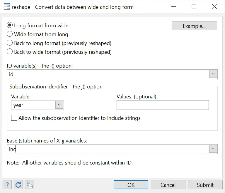
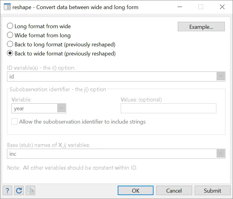
In the dialogue box that opens, four things need to be specified:

There are four things you need to specify here:

First, choose the type of reshape that you would like your data to undergo. Here, we want our data to go from wide format to long format, so we choose the very first option from the four checkboxes given.

Secondly, choose the unique identifier of your current data. This can also be a combination of variables. Here, it is just the ‘id’ variable.

Thirdly, specify the name of the variable that you would like to be created so that your data would go from wide to long. Here, we have three separate variables for each year’s income with their names prefixed with ‘inc’ followed by the year. To make this wide data format into a long format, we want that instead of three separate variables for each year’s income, we have only one variable called ‘year’ that stores the respective year for each id’s income. So, in the j() option (or the sub observation identifier), we type in ‘year’ so Stata creates a new variable with this name.

Connected to this, we lastly specify our stub which would also be used to change the data from wide to long. Here, the stub is ‘inc’. Stata will take all variables prefixed with ‘inc’ (‘inc80’, ‘inc81’, ‘inc82’) and combine them into one variable called ‘inc’. This new variable will then have all the years that were previously represented by separate variables.

The dialogue box, when filled, would look like this:

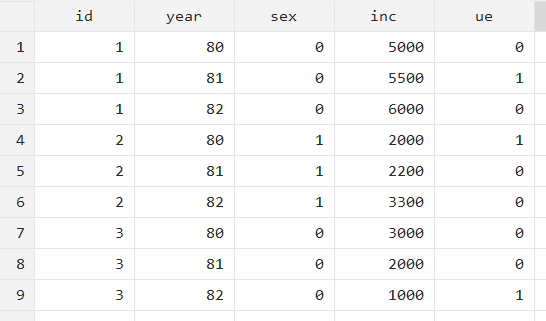
When you submit these entries, your data will be reshaped to long format and look like the following.

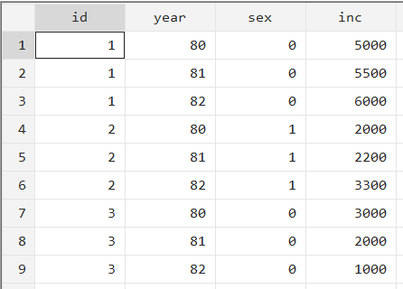
There is one variable for year now which means that for each ‘id’, there will be three observations: one for each year. The ‘inc’ variable will hold the corresponding income value for a specific id in a specific year.

Stata also returns us a summary of what the reshape command did to the data:

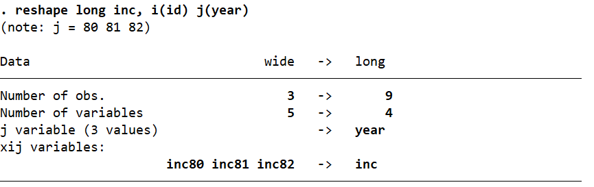
Firstly, it tells us that in reshaping the data from wide to long, we went from 3 observations to 9, and from 5 variables to 4. The j() variable with three unique values is called ‘year’, while our stub (xij variables) were three ‘inc*’ variables in the wide format (‘inc80’, ‘inc81’, ‘inc82’).

Going back to the original wide format after reshaping it to long is straightforward. Simply go back to the same dialogue box, and choose the “Back to wide format (previously reshaped)” option. Note that this will only work if you have already just reshaped your data from wide to long.

The syntax for the reshape in the above examples would look like this:

reshape long inc, i(id) j(year)

The reshape command is followed by long or wide, depending on what you want your data transformed to followed by the stub name (‘inc’). The unique identifier, i(), and the j() option are specified after a comma as options.

Note that even if you don’t specify the j() option when converting to long format, the command would still work and create a new variable with the relevant year data. However, Stata would name the new variable ‘_j’, so it is more convenient to add the option to indicate what we want the new variable to be named as.

In order to go back to the wide format, the following command would do the trick (but only in the case of a previous reshape long command):

reshape wide

Reshaping For Multiple Variables

We will now see how data can be reshaped when the structure is determined by multiple variables. In our previous example, we only had the income variables to work with. What if there are more variables that need to be taken into account. Let’s reload our dataset:

webuse reshape1, clear

This time, we keep the unemployment variables that we dropped previously (‘ue80’, ‘ue81’, ‘ue82’).

The only difference in reshaping this data to long format as compared to the previous one will be the addition of another stub name, in this case ‘ue’ for the unemployment variables. The options, as before, will include the i() option for the cross-sectional (unique) variable, and the j() option for the new variable to be created.

Similarly, the only difference if you use the command window will be the addition of a new stub name.

reshape long inc ue,i(id) j(year)

The data will be reshaped to long and look like this:

Again, to go back to the wide format, you can simply execute the command:

reshape wide

Reshaping Data With Numeric Variable Names/Headers

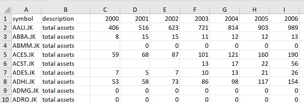
If your data has headers that are numeric, e.g. year names, it would be better to rename them with an alphanumeric name because Stata does not support purely numerical variable names. Data will have to be edited and imported from an Excel file. 

In our case, we have a wide-form data set that looks like this.

We will rename the column headers by adding a ‘Y’ prefix to the year names so that the headers become Y2000, Y2001,…, Y2006. In Excel, to do this quickly, you can first add a row on the very top of your sheet, and type ‘Y2000’ above the ‘2000’ field, and drag it horizontally. Excel will automatically fill the remaining columns with appropriate years and the ‘Y’ prefix.

Copy and paste the variable names with the ‘Y’ prefix over the previous numeric names and delete the first row.

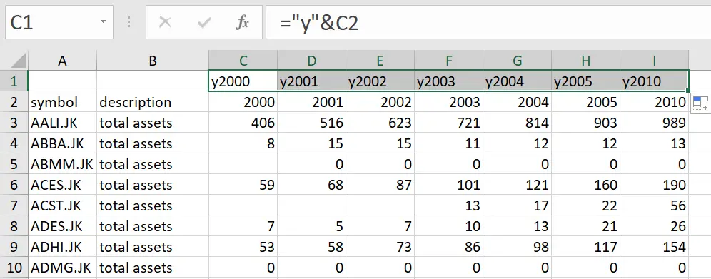
What if the year names are not sequential and the last column is for year 2010? Dragging the Excel formula will only produce column headers with an increment of 1. In this case, let’s employ a more dynamic formula that will automatically refer to which value is written under it, whether in sequence or not.

In the field above the year name, write the formula:

=”y”&C2

Here, C2 is the cell address where the first year of our data is mentioned. It may be different for you so write your formula accordingly. This formula produces the string ‘y’ (the inverted commas in the formula indicate that it is a string) followed by whatever is written in the cell you reference after the operator ‘&’. The operator ensures that anything mentioned before and after it is concatenated. In this example, it will concatenate the string ‘y’ and anything written in cell C2. When you drag the formula across the row, it automatically references the appropriate cell under rather than produce a specific prewritten value like before.

As you can see, the final column is now headed as ‘y2010’ because the formula references cell I2 to combine with the prefix ‘y’.

When copy and pasting the first row into the second, take care to choose the paste ‘Values’ options so that it does not replicate the formula in this row.

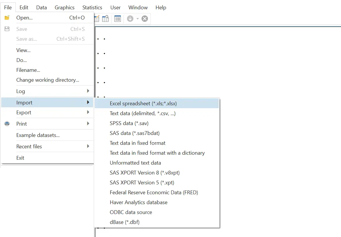
You can now import this dataset into Stata. To import an Excel dataset into Stata, simply follow the menu options:

File > Import > Excel spreadsheet (*.xls, *.xlsx) > Browse

Choose your Excel file and also choose the right sheet from the dialogue box that opens. Make sure to check the “Import first row as variable names” option.

Reshaping from wide to long is simple from here through the commands we used above.

reshape long y, i(symbol) j(year)

Our stub in this case will be ‘y’ for the ‘y2000’, ‘y2001’,…,’y2010’ variables. And though it is not necessary to specify the j() option, it is best to do so, so Stata can name the new variable for the stubs appropriately.

Reshaping With Multiple Unique Identifiers

We will now look at a scenario where multiple variables make up the unique identifier. Let’s load the reshape2 dataset.

webuse reshape2, clear

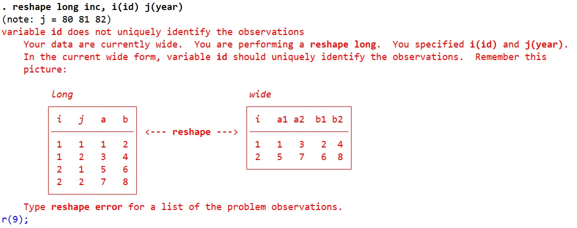
In the previous examples, we had only one variable like company name or someone’s id that uniquely identified each observation. Browsing this dataset makes it apparent that ‘id’ cannot be a unique identifier alone since ‘id’ == 2 appears twice. You can also check which variable(s) uniquely identify your dataset using the isid command.

isid id

This will return an error since ‘id’ alone does not uniquely identify the dataset.

isid id sex

Here, since the command returns no error, we know that the variables ‘id’ and ‘sex’ together identify each observation uniquely. We will therefore mention both of these variables in the i() option.  

reshape long inc, i(id sex) j(year)

If you were to run the reshape command with just the ‘id’ variable specified in the i() option, it would return an error that says, “variable id does not uniquely identify the observations”

Related Article: Using Rename command to rename Variable in Stata

Reshaping Multiple Variables

We will use the time-series company dataset for this example.

import excel "reshape example data.xlsx", sheet("multiple variables") firstrow clear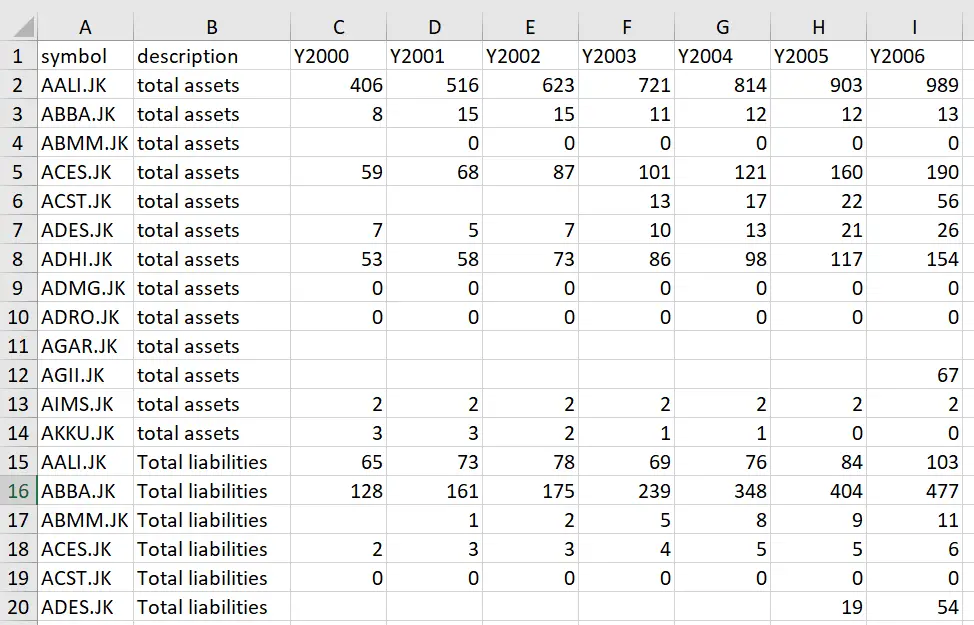

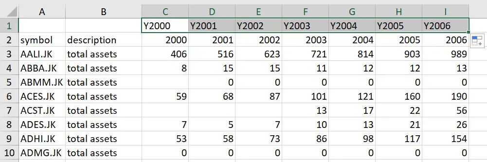
Note that for each company in the ‘symbol’ variable, there are two observations. This is because the ‘description’ variable takes on two values, “total assets” and “total liabilities”. Therefore there is one observation for the company’s total assets, and one observation for its total liabilities.

The rest of the variable names are just the variable names with a stub.

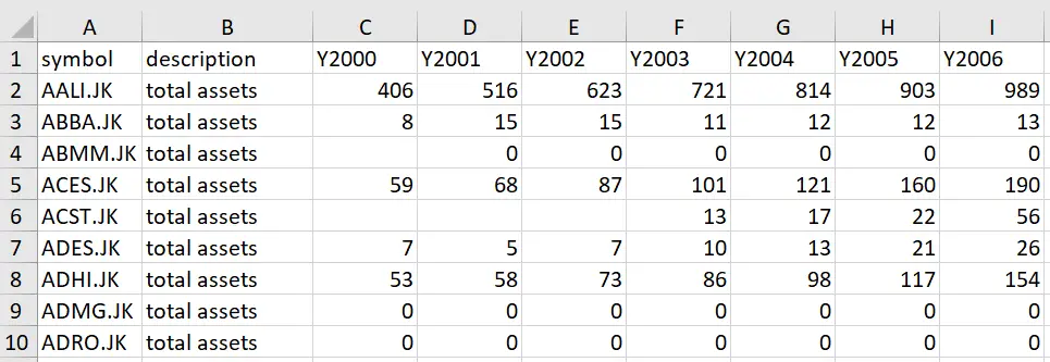
To create one variable for the years, we will reshape the data to long format.

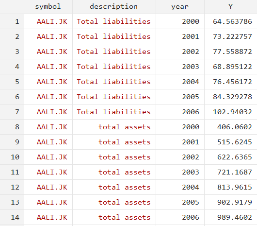
reshape long Y, i(symbol description) j(year)

We specify both the ‘symbol’ and ‘description’ variables as unique identifiers since they identify each observation uniquely as a pair – not on their own individually. Secondly, note that the stub name is a capitalised Y: variable names in Stata are case sensitive so we must be careful when referencing them.

The data will be reshaped as follows with just one variable for years.

Reshaping With String Variable Names

Finally, let’s see how we can reshape our data when our variable names are of the string type. Our dataset for this example looks like this:

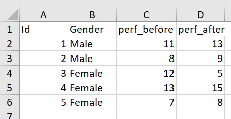
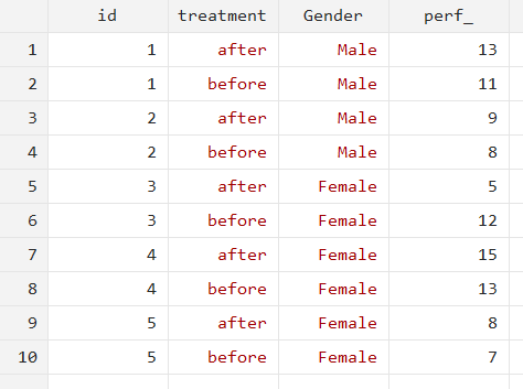
There are four variables called ‘Id’ which uniquely identifies an employee of a firm, ‘Gender’ which specifies their gender, and ‘perf_before’ and ‘perf_after’ that quantify the employees’ performance before and after a treatment respectively. All the variables are named as strings.

The dataset can be imported into Stata using a command or the menu options:

import excel "reshape example data.xlsx", sheet("string header") firstrow clear

As can be seen, the data is in a wide format right now. In order to convert it to long form, we once again specify the stub, unique identifiers and the j() option for our reshape command. The stub name should be chosen/written in a way while keeping in mind how our reshaped data should look. In this case, we want our observations to just say ‘before’ or ‘after’ for the new variable called ‘treatment’. Because the variable names ‘perf_before’ and ‘perf_after’ have the prefix ‘_perf’, that is going to be our stub. Make sure the underscore is included in our stub; otherwise, the symbol would stay attached to ‘before’ and ‘after’.

We want to name our new variable that will be created after the reshape ‘treatment’, therefore we will specify this in our j() option.

A new option that will need to be added to the reshape command is string. This is to indicate that the new variable ‘treatment’ will be a string variable rather than the default numeric.

Another thing to remember is the case-sensitivity of Stata and the variables. Our unique identifier, i.e. the i() variable is called ‘Id’ with a capital ‘I’. If you were to write i(id), Stata would return an error and fail to run the command since it won’t find any variable called ‘id’ in the data. ‘Id’ would be the correct way to refer to the variable. To avoid this problem, it is usually better to name your variables in lower-case letters.

In our dataset, ‘Id’ and ‘Gender’ have their first letters capitalized. A quick way to convert your variable names to lower-case is to run the following command:

rename Id Gender, lower

These variables are now renamed to ‘id’ and ‘gender’. We can run the reshape command now.

reshape long perf_, i(id) j(treatment) string

Our data will be reshaped as follows:

For each ‘id’, there is one value each of ‘_perf’ before and after treatment. This treatment status is shown by the newly created ‘treatment’ variable that takes on a value of either ‘before’ or ‘after’.

Numerical Variable Names With Special Characters

Finally, we will look into how data can be reshaped when the variable names/column headers have special characters in their names.

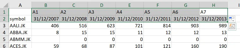
For this example, we will use a dataset of yearly stock prices that looks like this:

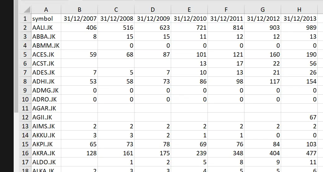
For each stock under the ‘symbol’ variable, there is one observation. The observation contains its stock price on the 31st of December of year from 2007 to 2013. These dates are our column headers. These dates have special characters (/) and thus Stata would not accept them as variable names.

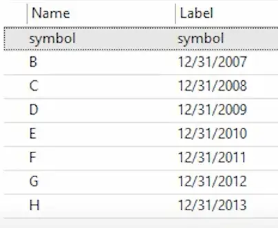
If you do import this data as it is into Stata, Stata will change the variable names to B, C, D,…,H and keep the original column headers as labels.

To get around this issue, we will follow the following steps. The steps are divided into two parts: ‘Part 1: Excel’ and ‘Part 2: Stata’:

Part 1: Excel

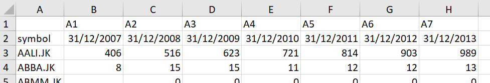
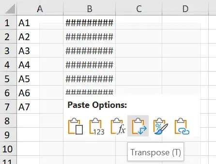
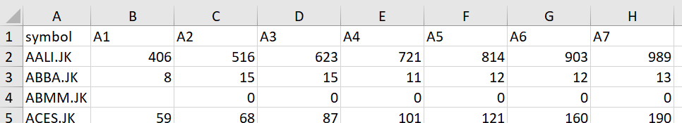
1. Add a row at the top of the Excel sheet and write an alphanumeric name above every date. We will simply use the prefix ‘A’, followed by a number sequentially.

2. Select the top two rows (only those cells with the dates and the new alphanumeric names) and copy them.

3. Create a new sheet called “change name”. Choose the ‘Transpose’ option when pasting this copied data. Transpose changes columns to rows, and rows to columns.

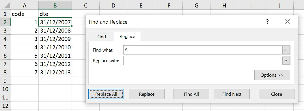
4. Name the first and second columns as ‘code’ and ‘date’ respectively.

5. Remove the ‘A’ prefix from the first column using the ‘Find and Replace’ feature in Excel.

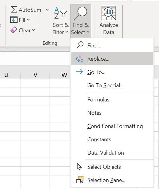
6. Replace ‘A’ with a blank so your sheet now looks like this:

7. Go back to the original sheet with the stock price data, and replace the date column headers with the corresponding A1,…, A7 headers you added above them. This will just entail simply copying and pasting the headers onto the old date headers and removing the first row. Your data would look like this now:

Related Article: Data Frames in Stata | Store Multiple Datasets in Stata’s Memory

Part 2: Stata

1. Import the ‘change name’ sheet into Stata. You can use the menu options or the command:

import excel "reshape example data.xlsx", sheet("change name") firstrow clear

2. Save it, as it is, in .dta format. Make sure the first row is imported as variable names. You can save this data either via the menu options: File > Save As

or

by typing in the save command followed by your desired file name with a .dta extension:

save change_name.dta

3. Import the original stock price dataset into Stata. Use the clear option if you still have some existing dataset in your Stata window. You can use the menu options or the command:

import excel "reshape example data.xlsx", sheet("special character header") firstrow clear

We have once again imported the first row as variable names.

4. Reshape this data. Note that the variables that originally had dates as their names are now named as ‘A1’,…, ‘A7’. The prefix ‘A’ would thus be our stub. And since each stock symbol has only one observation, ‘symbol’ is our unique identifier. We will name the new variable, i.e. the j() option as ‘code’.

reshape long A, i(symbol) j(code)

The reshaped data would look as follows:

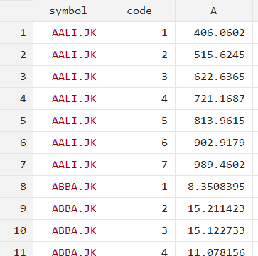
There are multiple observations for each symbol now since each row represents the stock’s price on one specific date.

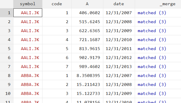
5. Merge this dataset with the change_name.dta dataset that was saved earlier. This can be done by following the menu option: Data > Combine datasets > Merge two datasets > Check “Many-to-one on key variables (unique key for data on disk)” > Enter ‘code’ in the field called “Key variables: (match variables)” > Click “Browse” > ’Select the ‘change_name.dta’ file

You can also use the command:

merge m:1 code using "change_name.dta"

6. Sort your data by ‘symbol’ and ‘date’ using:

sort symbol date

Your data will look like this now. Each symbol will have its stock price on a certain date stored in one observation.

7. Drop variables that are no longer needed. You may also rename ‘A’ as you like.

drop code _merge rename A price

Reshaping to Wide

If you just reshaped your data to long form, you can simply use the command reshape wide to revert it back to its wide form.

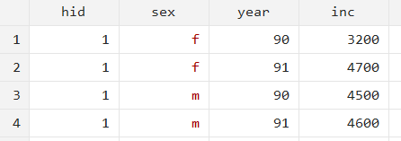
In order to practise reshaping a long form dataset from scratch, let’s use the “reshape5” dataset.

webuse reshape5.dta, clear

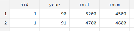
This short dataset has 4 observations, each with the same value for ‘hid’, two categories for ‘sex’, a variable for ‘year’ which also has only two unique values, and a variable called ‘inc’.

Since the cross-sections (a combination of ‘hid’ and ‘year’) repeat longitudinally, we can convert them to wide form so that there is only one observation for an ‘hid’’s income.

In the case of reshaping from long to wide, the j() is an existing variable. And though it is evident, you can always check the unique identifier through the isid command:

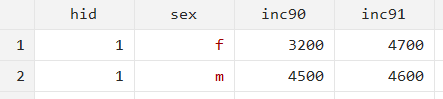
isid hid year reshape wide inc, i(hid year) (sex) string

This results in:

Note that it has created one variable for females’ income (‘incf’) and one for a males’ income (‘minc’).

We can tweak the command a little to get a different kind of wide-form data. What if one male and one female could have the same ‘hid’? Instead of having a single variable for year, and having the income variables separated by gender, let’s try achieving a single variable for gender, and the income variables separated by years.

reshape wide inc, i(hid sex) j(year)

This will result in:

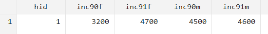
You can make this data even “wider” if you like by combining both the ‘sex’ and ‘year’ variables with the income variable.

reshape wide inc90 inc91, i(hid) j(sex) string

The data will now have only observation for each ‘hid’. The income variables (inc*) will indicate the gender and the year.