The Basics of Event Study

An event study investigates how an event affects a security’s value, such as stock price, trading volume, or return volatility. The response of security to any event can be predicted with the help of event studies. The fundamental idea underlying event studies is that a company’s stock price reflects all known information, including public and private information. Any new information, such as a merger or earnings announcement, will have a predictable impact on the company’s stock price. Researchers can determine the size of the impact of an event on the company’s financial indicators by analyzing the stock price movement surrounding that event.

An event can be classified as macro-level, firm-specific, or industry-specific. Some examples of events that could majorly impact a business or industry are mergers, acquisitions, earnings announcements, dividend announcements, stock split announcements, or regulation changes. In finance, we measure the impact of these events, specifically on the stock price or stock index. The event study is carried out in five steps.

Related Article: Estudy Command for Event Study in Stata

Step 1: Identify the event of interest

The first step in the event study is to identify the event we are interested in and investigate its impact on any stock or index. This also includes selecting the company likely to be affected by the chosen event. This step includes, gathering data pertaining to the stock prices during a designated time frame, preceding and succeeding the event’s occurrence. For example, the event we are focusing on is the date of a stock split announced by Apple Inc. We need to identify the date of a stock split and the company’s stock price before and after the event.

Step 2: Deciding the estimation window

The estimation window in an event study is the time frame used to compute the expected or benchmark return for a stock or index. This time period starts before the event and ends before it happens. Therefore, the second step is to determine the event window. This window can be for a different time period, such as:

1. 150 days
2. 225 days
3. 239 days

It is solely based on the topic of research. It is a must to choose the event window carefully for each unique occurrence and security due to two main reasons. First, a too-small window won’t capture security’s typical behaviour. Second, a too-large window will include outlier periods that do not represent the actual picture of a security’s normal market behaviour.  

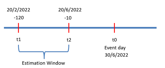
For example, on June 30, 2022, Apple announced its stock dividend. The estimation window is the time before that event. In the above figure, t1 and t2 represent the time periods of the estimation window. The estimation window starts on February 20, 2022, and end on June 20, 2022, 10 days before the event and continues till 120 days before the event. The question is why it does not start one day before the event but ten days before it. Some events might have an effect before their actual occurrence. It is a must that the estimation window includes the days that are free from the effects of the event.

Step 3: Deciding the event window

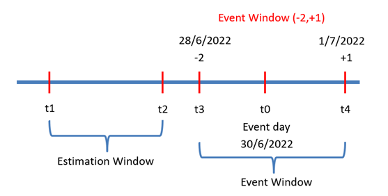
            In the third step of the event study, we calculate the return for the event window. The event window is the time around the event, also known as the test period. The influence of the event on the stock is examined during this window. During this period, actual or abnormal returns are calculated. The t3 and t4 in the figure below represent the event window (-2. +1). Two days before and one day after the event.

The purpose of this event window is to determine when the stock is over or reacts because of the occurrence of an event. Some of the event windows are listed below:

• (0,1) One day after the event
• (0,5) Fiver days after the event
• (-1,0) One day before the event
• (-2, +2) Two days before and two days after the event

Related Article: Event Study using the Eventstudy2 command in Stata

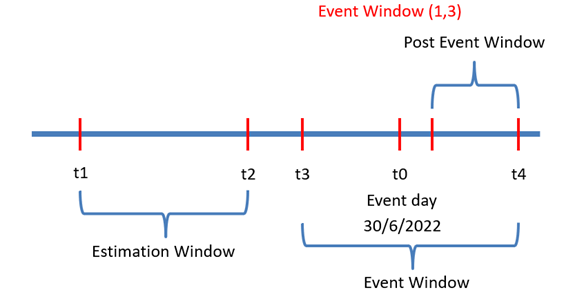
The event window can also be a post-event window like (1,3). The post-event window does not include the days before the event and the day of the event. After this, we will calculate the abnormal return, the difference between the actual and expected returns. For instance, if we assume the event window (-2, 1), we will calculate the actual return for two days before, one day before, the day after the event, and one day after. Once we get the actual return, we will subtract them from the expected return calculated in step two.

Step 4: Estimating Expected Returns

The estimated return on the event date is computed during the estimation window using different models. Historical data is utilized to forecast the return on the day of an event. The models are discussed below:

1. Mean Adjusted Return

In this model, we take the average of the stock return from the time period February 20, 2022, until June 20, 2022 (estimation window = 120 days). For instance, if we get an expected return of 1.25%, we will say that on the event date, the return will likely be 1.25%. The formula for mean adjusted return is given below:

2. Market-Adjusted Return

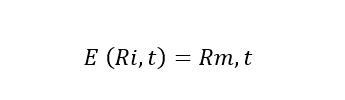
According to this model, the expected return equals the market return on the event date. The utilization of the market-adjusted return approach does not necessitate the need for an estimation period.

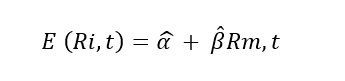
3. Market Model

It is typical practice in event studies to utilize the market model to evaluate the expected return. The computation of the expected return is predicated upon a market model incorporating one single factor. The estimation period is utilized to estimate the parameters of the market model precisely and through the application of Ordinary Least Square (OLS) regression. The approach is utilized to regulate the relationship between the returns of a given stock and the returns of the market or to account for the risk fluctuations linked to a particular stock. The anticipated return, adjusted by the market model, is frequently observed as a typical return in prior event analyses.

Related Article: How to Calculate Stock Return in Stata

4. CAPM

Given an asset’s beta, the risk-free rate, and the expected market return, the model calculates the asset’s expected return, and this method is known as CAPM. The Capital Asset Pricing Model (CAPM) posits that the expected return is a function of the risk-free rate of return and the market risk premium. The model assesses the level of risk associated with a particular stock under the assumption that an investor demands a greater return to offset more significant risk. To use the CAPM, one should know the risk-free rate, the beta, and the predicted market return.

5. FF3 Factor Model

The expected return on a stock can be calculated using the Fama-French Three-Factor Model (FF3). Market risk, company size, and stock valuation are the three primary components of the FF3 model, which is used to predict stock returns. It is a must to know the risk-free rate, market return, size premium, and value premium before applying the FF3 model. The stock’s projected return under consideration can then be estimated by calculating the betas for each element using historical data and plugging those values into the formula.

In the above model, Small-minus-big (SMB) refers to the difference in average returns between portfolios of small and large stocks. The High minus Low (HML) factor pertains to the difference in mean returns observed between portfolios of stocks with high and low book-to-market ratios. The approach employed involves the utilization of monthly returns covering a long time period.

Step 5: Calculating the CAR or BHAR

• Cumulative Abnormal Return (CAR)

The measure employed in event study analysis to assess a specific event’s effect on a stock’s performance during a designated time frame. The Cumulative Abnormal Return (CAR) measures the total return earned by an investor who retains a stock from the start of the event window until the end of a designated post-event window. The abnormal return will be calculated for each day. In an event study, we need aggregate return over the event window. Therefore, we will take the average of each day’s abnormal return over the event window. This return will be known as the Cumulative Abnormal Return (CAR). The CAR formula is given below:

This CAR value tells us how the event has affected the stock market or a specific stock return.

• Buy and Holds Abnormal Return (BHAR)

Investors buy a stock at the start of the event period and sell it at the end of the event period. The BHAR measurement denotes the cumulative abnormal return that an investor obtains by purchasing a stock at the onset of an event window and retaining it until the end of the window.

• Cumulative average abnormal return (CAAR)

            For instance, if we have ten different events on different dates. We will calculate the CAR for each event type or category. The average of all these CAR of different events will be known as the CAAR.

Step 6: Significance of AR and CAR

            The last step in the event study is to test whether the AR and CAR are equal to zero. To test this, a t-test will be carried out. There are two types of t-tests parametric and non-parametric.

• Parametric Test:

Parametric t-tests are a type of statistical analysis employed to ascertain a significant difference between the means of two distinct groups. The analysis assumes that the data conforms to a normal distribution and that the variances of the two groups under comparison are equivalent.

T-Test

• Non-Parametric Test:

Non-parametric tests are the opposite of parametric t-tests. It is also employed to ascertain the presence of a significant difference between the means of two distinct groups but when data failed to conform to a normal distribution and that the variances of the two groups under comparison are not equivalent.