Export Summary Statistics, T-tests, and Tabulations from Stata.

In our previous article, we discussed how to export the results of regression analysis from Stata to MS Word or Excel. In this article we will explore how to export results from Stata to Excel or Word formats. We’ll cover exporting summary statistics, performing mean comparison tests (t-tests), and generating one way and two way tabulations.

Initial Preparations:

Download Example File

The estout command can be installed on Stata through the

ssc install estout

command. The installation takes a few minutes. Remember to keep the command

help estpost

in memory, as it can help you with commands whenever you are stuck.

We also need to load our auto data set by

sysuse auto.dta

command. After that, we are ready to move forward.

Exporting Summary Statistics from Stata:

E-class Verses R-Class Commands:

To understand the difference between the two types of command is necessary. E-Class Commands are primarily the estimation commands such as performing regression analysis. They focus on estimating model parameters and generating associated statistics. However, E-class commands alone are not designed to provide summary statistics like means, standard deviations, and medians directly.

On the other hand, R-Class Commands are class commands specifically intended for generating summary statistics and other analytical measures including correlations, tabulations.

eststo Verses estpost:

Both of these commands are from the family of ‘estout’ command. But, for exporting summary statistics, we use the ‘estpost’ command instead of the ‘eststo’ command.

Generating Summary Statistics

To obtain summary statistics, we use the ‘summarize’ command followed by the variable names. An example of such command would be,

summarize price length rep78

By adding ‘estpost’ before ‘summarize’, i.e.

estpost summarize price length rep78

we can store the statistics in Stata’s memory for further use and export.

Selecting Summary Statistics

We can choose the desired statistics to Auto display by using the ‘cells’ option. For example, in the command,

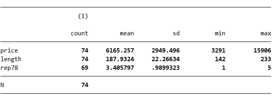
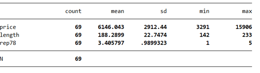
esttab , cells(“count mean sd min max”)

the cells will select count, mean, standard deviation, minimum, and maximum values to export. An illustration is given below to show you what to expect from this command,

Using Detail Option for Additional Statistics

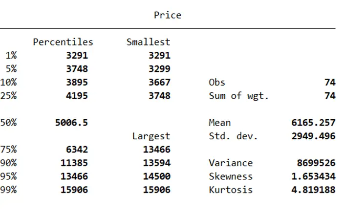
Summarize command can be used in two ways. The first way is our familiar one; using it to summarize our variables. On the other hand, adding the ‘detail’ option to ‘summarize’ allows us to access more statistics like percentiles, mean, median, skewness, and kurtosis. An exemplary command for this particular action is,

summarize price, detail

The illustration shows the detailed statistics of the variable of price.

So, the following command would show detailed statistics of the variables of price, length and repair record of 1978:

estpost summarize price length rep78, detail

Using Skewness in Detail Option:

However, it is necessary to know that these details, shown below, require using ‘estpost’ before ‘summarize’ in a command to work.

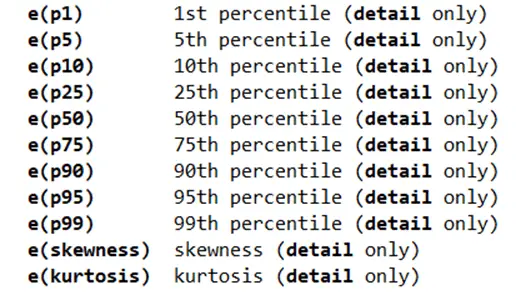
As the detail option is used in the previous command, you can now work with skewness through this command,

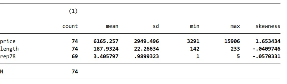
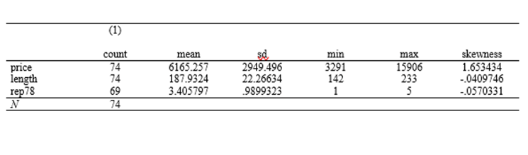
esttab , cells(“count mean sd min max skewness”)

Your result will show a column for skewness, as such

Exporting Summary Statistics:

Export the summary statistics to Word or Excel using ‘esttab’ command along with the appropriate file names. To export in MS Word, use rtf (Rich Text Format) as such

esttab using result.rtf, cells(“count mean sd min max skewness”)

Your data will be exported to an MS Word file titled, ‘result’

For exporting in MS Excel, use csv (Comma separated Values) as such

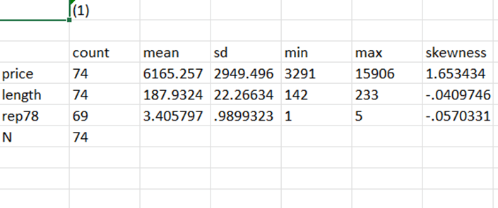
esttab using result.csv, cells(“count mean sd min max skewness”)

Your data will be exported to an MS Excel file titled, ‘result’, i.e.

You can also use the desired formatting options. The listwise option makes sure to exclude observations with missing values from the analysis. When you use the listwise option, those observations will be completely omitted from the calculation. This is often used to ensure that only complete cases are considered in the analysis.

An example for such command is,

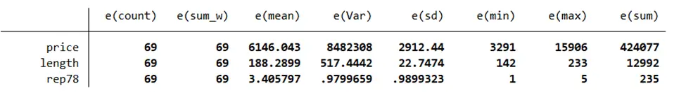
estpost summarize price length rep78, listwise

Your data will look like this,

The casewise option is useful for handling the missing values on a variable-by-variable basis. When you use the casewise option, Stata calculates statistics only for the rows/cases where the entire record is available i.e. data for all the variables price, length, rep78 is available. This specifically means that an observation will not be included in the analysis if it has missing values in any other variables.

Other ways for formatting outputs can have options such as ‘noobs’, ‘nonumber’, and column labels called the ‘mtitles’. They customize the output to your liking. Your model commands for these actions would be,

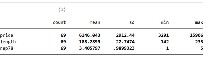
esttab , cells(“count mean sd min max”) noobs

This would remove the observations as such

nonumber and nomtitle opiton will remove then number at the top and the titles,

esttab , cells(“count mean sd min max”) nonumber nomtitle

would remove m titles and number as shown below,

Generating Summary Statistics by Group:

We can generate summary statistics for different groups of variables. The ‘foreign’ variable explains whether the car is foreign or domestically produced. For this ‘foreign’ variable, let us say, we need separate summary statistics for each category. Our command should be

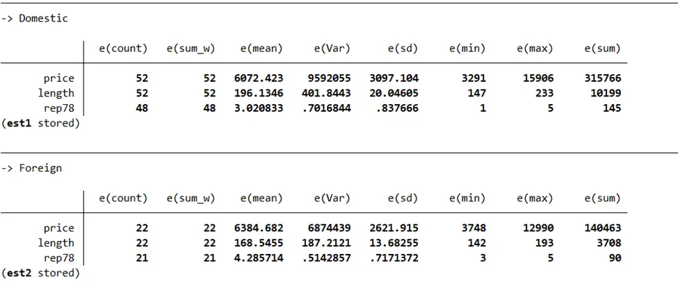
by foreign: eststo: estpost summarize price length rep78

Your output window will show categorical summary statistics for this variable as such,

You can get the mean and standard deviation of the data above with

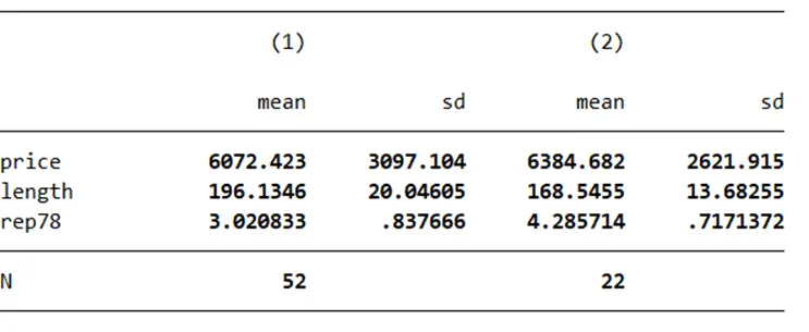
esttab, cells(“mean sd”)

command. Upon execution, you would be able to see this,

You can customize this output too. With a command

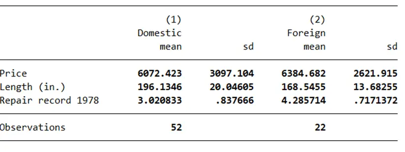
esttab, cells(“mean sd”) label nodepvar

your data will look like this,

Exporting Main Comparison Test Results (t-tests)

Performing t-tests

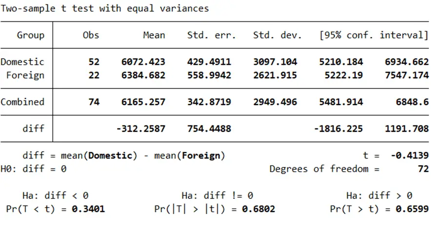
We need to perform t-tests to compare means between certain groups. For example, to compare car prices for domestically produced and foreign cars. The command for this specific example would be,

ttest price, by(foreign)

This will show two sample t-tests with equal variance with a statistically insignificant t-value.

Using estpost with t-tests

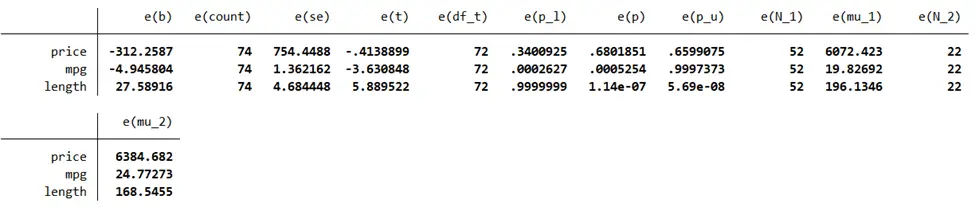
While t-tests typically require separate commands for each variable, using ‘estpost’ as a prefix allows us to perform t-tests for multiple variables in one command. You can add multiple variables in the same command to compare the domestically produced and foreign cars. Thus, the command,

estpost ttest price mpg length, by(foreign)

will provide the mean comparison for price, mileage and length for foreign and domestic cars,

Interpreting t-test Results

T-test results provide mean differences and t-values. We can assess statistical significance and differences between variables for different categories.

Exporting t-test Results

To export t-test results, use ‘esttab’ with desired formatting options. A command,

esttab .

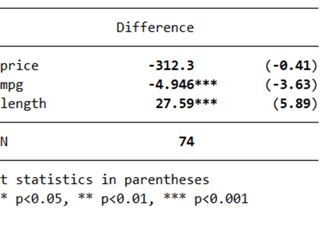
will produce the results that can be exported too. The wide option, along with other custom options, in the command

esttab .,wide nonumber mtitle(“Difference”)

will allow for clean and organized output that can be saved in Word or Excel format.

Command for one Sample or Paired t-test:

For one sample t-test or Paired t-test, the command, ‘estout’ does not work easily. Thus, we need to use ‘asdoc’ command.

Exporting Tabulation Results

One-Way Tabulations

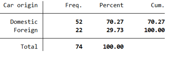
One-way tabulations are involved in calculating frequencies and percentages for a single categorical variable. For example, the command

tabulate foreign

will provide frequencies and individual and cumulative percentages, as shown below

Using estpost with One-Way Tabulations

Similar to previous cases, we use ‘estpost’ before ‘tabulate’ in our command to export the tabulation results. Thus, your command, following the previous examples, would be,

estpost tabulate foreign

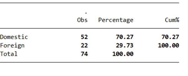
However, this command will only provide you frequencies and not the percentages. Here, ‘cells’ option can be used to customize the output. To ensure you get the percentages along the frequencies, you can use the following example of the command,

esttab ., cells(“b(label(Obs)) pct(fmt(2) label(Percentage)) cumpct(fmt(2) label(Cum%))”) noobs nonumber nodepvar

Your results will be,

Exporting One-Way Tabulations

Export the tabulation results using ‘esttab’ while specifying desired columns, labels, and formatting options as shown above.

Two-Way Tabulations

Two-way tabulations involve analyzing the interactions between two categorical variables.

Using estpost with Two-Way Tabulations

Again, use ‘estpost’ before ‘tabulate’ in a command for two-way tabulations. For example,

tabulate rep78 foreign

Exporting Two-Way Tabulations

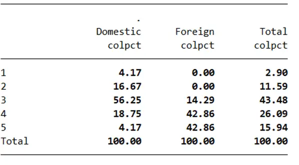
Similar to one-way tabulations, export two-way tabulation results using ‘esttab’ while specifying the desired formatting. Adjust formatting options and use ‘unstack’ to refine the output. An example for such command is,

esttab ., cell(colpct(fmt(2))) unstack noobs nonumber nodepvar

will show the following results, ready to export.

By now, you can export summary statistics, t-test results, and tabulations efficiently. Customizable formatting ensures clear and well-presented results for use in publications or reports. Remember to always explore several options and refine your export based on your analysis needs. Happy Learning!