
We will delve into the process of exporting status results to either an Excel or MS Word file. This facilitates the execution of specific analyses, allowing us to conduct detailed assessments. The crux of the matter lies in effectively exporting these outcomes in a table style suitable for publication. Our current focus is dedicated to comprehensively understanding and utilizing the “estout” command. This command is essentially a package of commands designed to encompass a range of analytical functionalities.
Throughout these analytical functionalities, we will explore how to apply this command set to various types of analyses, such as regression analysis, summary statistics, mean comparisons, one-way tabulation, and two-way tabulation. Our primary goal is to comprehend each analysis and seamlessly export its outcomes to Excel or MS Word files.
Getting Started with estout:
To begin, let us initiate the installation process of this command by utilizing,
Download Example Filessc install estout
By running this command, the installation will complete in a few minutes. Now, let’s proceed to load our auto dataset which includes data on various cars, such as price, mileage, weight, length, and whether they are domestically produced or foreign. To use the auto data, your command should be:
sysuse auto.dta
With that, we will be now able to initiate regression results.
Help Menu of estout Command:
To engage with regression results, consider consulting the help menu of the estout command. This command comprises of some sub-commands like “esttab,” “eststo,” “estadd,” and “estpost,” each serving their specific functions. The “estout” command is particularly comprehensive and detailed command. For working with regression, we will specifically utilize “eststo” and “esttab.” The former, called the est store command, stores the estimates in Stata’s memory, while the latter does twice the work, it displays the estimates as well as exports these estimates in the Stata output window. Also, the esttab command saves the estimates into an Excel or a Word file. Thus, this command is more unique than others.
Regression Analysis Results:
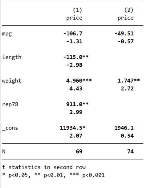
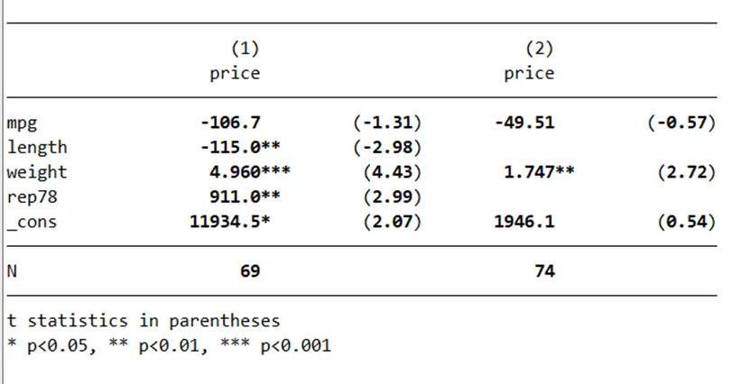
Let’s dive into the process. Let us say, our regression command is “regress price mpg length”. Running this command would help in showing the regression of variables of price mileage and length. It would show up something like this,
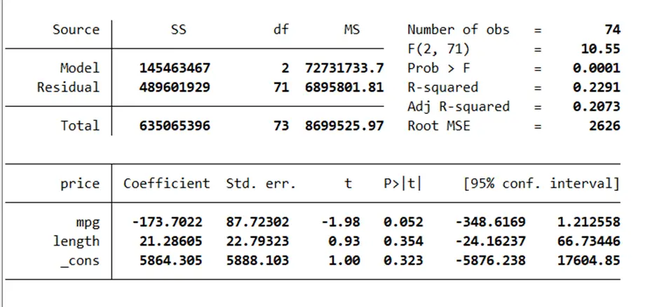
However we also need to store the estimates from the regression command. To do that, we need to append “eststo” as a prefix to this command. The command for running the regression and storing the estimates would be
eststo: regress price mpg length
This will store the estimates, leading to a message appearing in the status window.
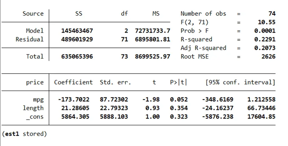
All of the regression from this command would bear the same results as the previous one, however, at the very end you would be able to see that the estimates are stored. To go a point further, the command
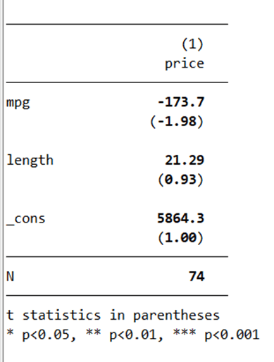
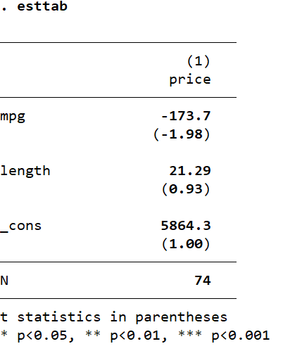
esttab
can be employed to display the results as they would be exported, exhibiting the estimates in the startup results window. Furthermore, the same command enables saving the estimates in either an Excel or MS Word file. This unique feature distinguishes “esttab” from other commands.
Now, let us examine regression with a different set of independent variables, such as weight. The command for such regression is,
regress price mpg weight
However, instead of using eststo as a prefix to a command, we can use it after the regression command. Additionally, we can add names that would be used to store the estimates. For the sake of example, we were working with the independent variable of weight in this specific regression. The descriptive name to store this regression should be executed as a command as such
eststo weight
While working with regression, the “esttab” command assists in displaying estimates and exporting them. These results are now stored and can be accessed using the
esttab
command. Your output window will show something like this,
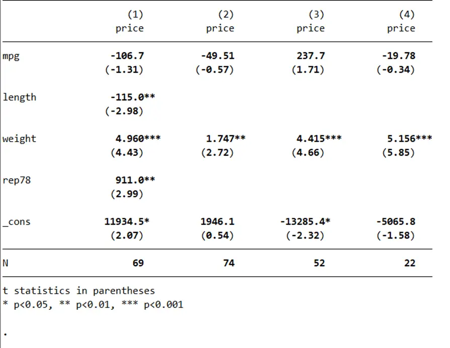
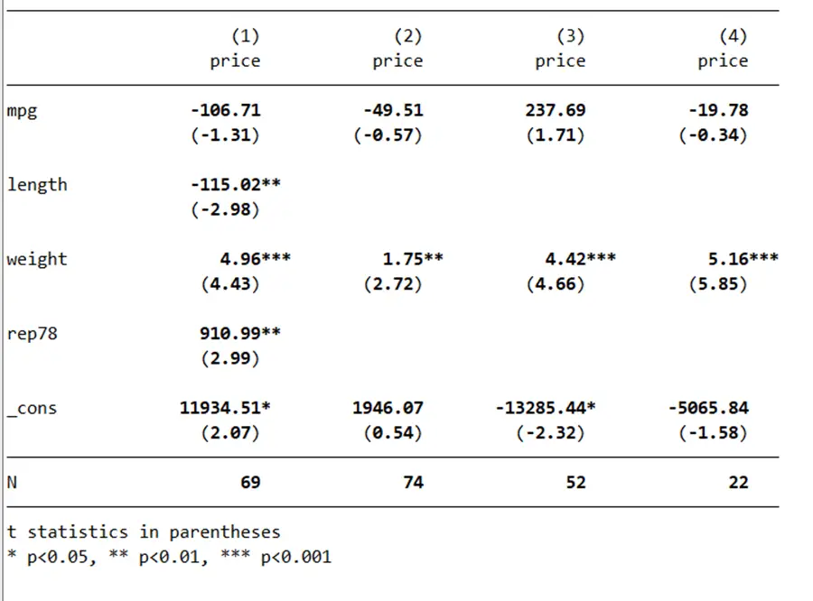
Continuing, we can perform further regressions, modifying independent variables as needed. It’s essential to understand that “eststo” can be employed in two ways: as a prefix for simultaneous storage or by specifying the name afterwards. The latter approach is useful for descriptive labeling, aiding recall of the stored results. Now, let us do another regression where we use the following command
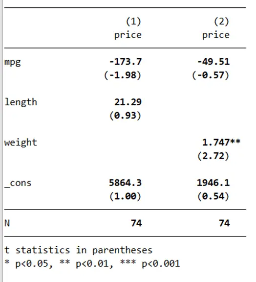
eststo both: regress price mpg length weight
By using the command,
esttab
We can display the results as such,
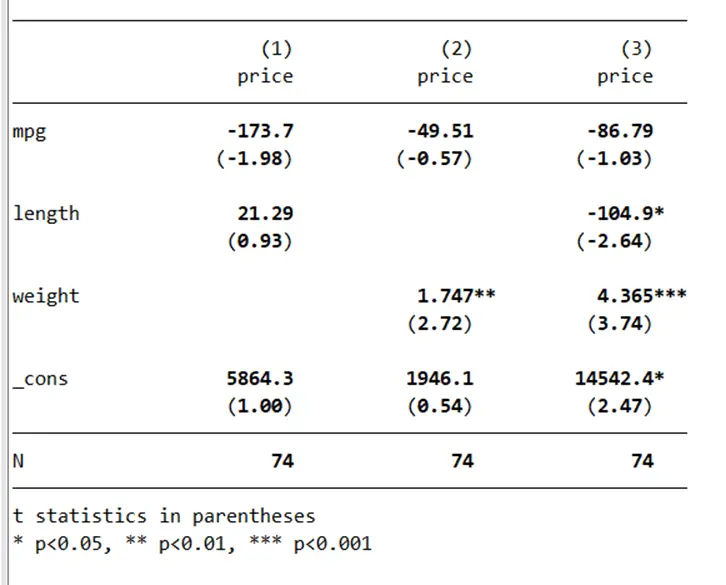
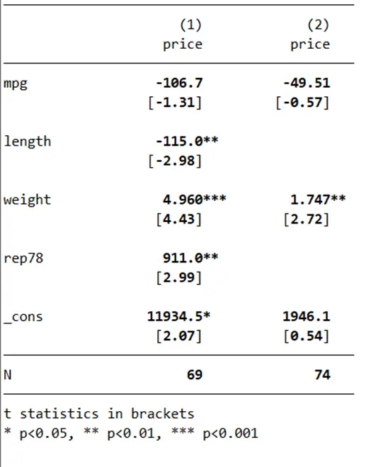
To know how these columns of “price” can be changed and how we can have standard errors in parenthesis, you need to stick with us. These issues will be addressed soon in the article, stay tuned!
Exporting Results to Different Formats:
Now, we need to explore more advanced options for exporting the results in an MS Word File, you need to work this command
esttab using results.rtf
If you want to save your results in an Excel file, your command would be
esttab using results.csv
You can identify that both of the commands are identical, instead of the suffix attached to them after the period. To keep them in mind, “rtf” would be used when you are trying to save results in Word File and “csv” if your desired file is Excel.
So, let us assume that we wanted to save it in a MS Word file. You can see from the Stata output window, that the “result.rtf” looks like a link.
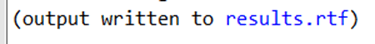
You can access the file by clicking on it and it would open an MS Word document, titled “results”, and would show something like this,
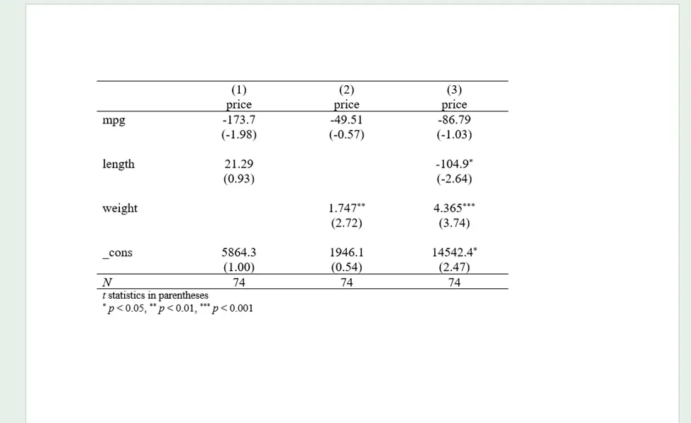
You can format these exported results.
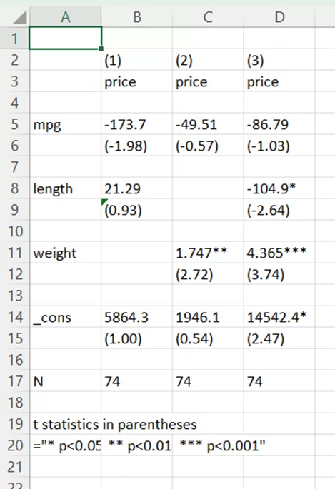
Let us assume that we wanted to see it in Excel too. After running the above mentioned command for Excel, you can see your results in the Excel file as such,
You can also save your files in latex format by using “tex” as a suffix. To clarify, your command would be
esttab using results.tex
Options with eststore command:
Let us explore the options for eststore commands.
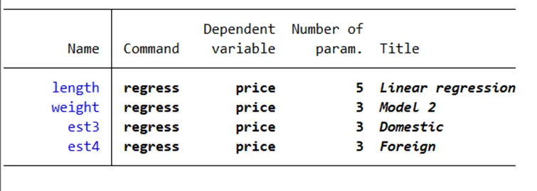
The
eststo dir
command presents a directory of all the stored results. By executing this command you can see the stored results as such,
Note that the names of these results are customized to our liking. The result table is also showing the executed command, the dependent variable, the total number of parameters we had, and the title. You can also see that the names of our results are colored blue, which helps us identify that these are clickable to open further details. For the sake of example, if I click on our first result ‘est1’, this would pop up,
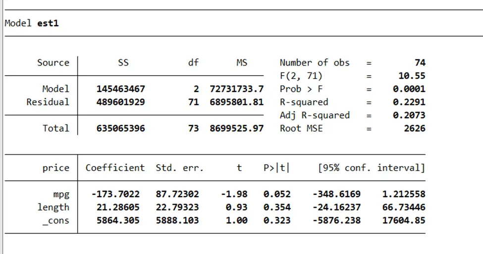
This replays the estimated results for ‘est1’.
To drop stored results, “eststo drop” followed by the result name is employed. For example, we need to drop ‘est1’, our command would be,
eststo drop est1
By executing this command, you can see ‘est1’ drop simultaneously.
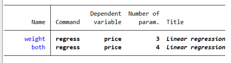
If you look at the directory now, you will see that ‘est1’ has been dropped from saved results.
Multiple results can be dropped at the same time as well. Thus, the command
eststo drop weight both
Would delete both of the results from the directory and the directory would be left empty. To check the directory, the command
eststo dir
would show blank output.
We can also drop all stored results through one command, i.e.
eststo clear
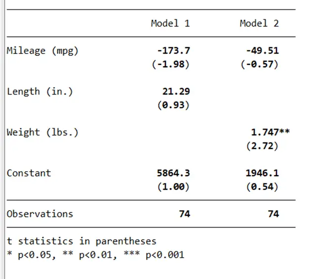
Customization is another key aspect. Titles can be modified to reflect the content of the stored results. To change the title for the stored results, we first need to generate new results to work upon. Through the command,
eststo length, title(“Model 1”): regress price mpg length
Here, we have specified the title. This option is available with the eststo command. You need to add the title after the comma and before the colon, your desired command would come after the colon along with the variables used. Let us derive another result from this command,
eststo weight, title("Model 2"): regress price mpg weightAfter execution of this command, we can simple execute the
esttab
command to get these results,
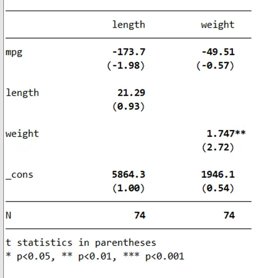
You are right to notice that even if we have specified the titles for our results, they are not displayed when we execute our esttab command. The reason for that will be: it would always display the name of the dependent variable, by default. To prevent this from happening, we can use the command,
esttab, nodepvar
This command would guide the results to not display the names of the dependent variables. Rather it will show the name of that stored regression result.
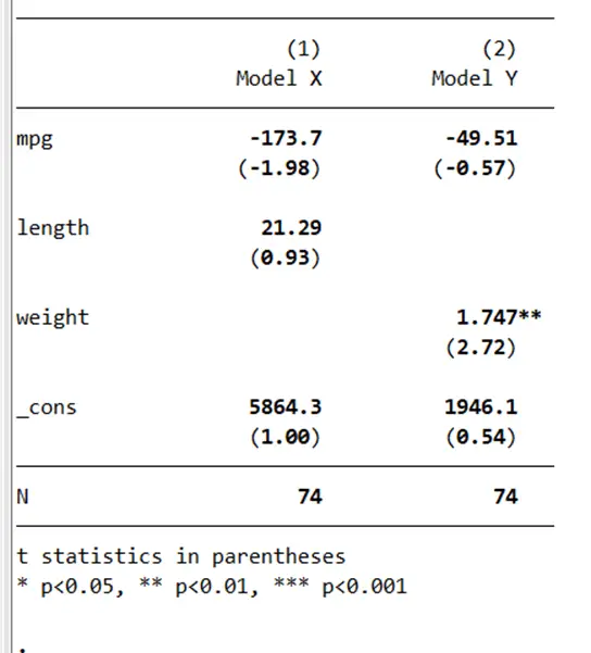
If you do not want the numbers displayed on top of the names of the results, i.e.
You can run a command,
esttab, nodepvar nonumber
Your results will show up like this,
Let us assume, that we also want the title to be shown in the results, instead of the names of the results. For that, we can execute the command,
esttab, nodepvar nonumber label
And you can clearly see in your Stata output window that the names are replaced with the titles,
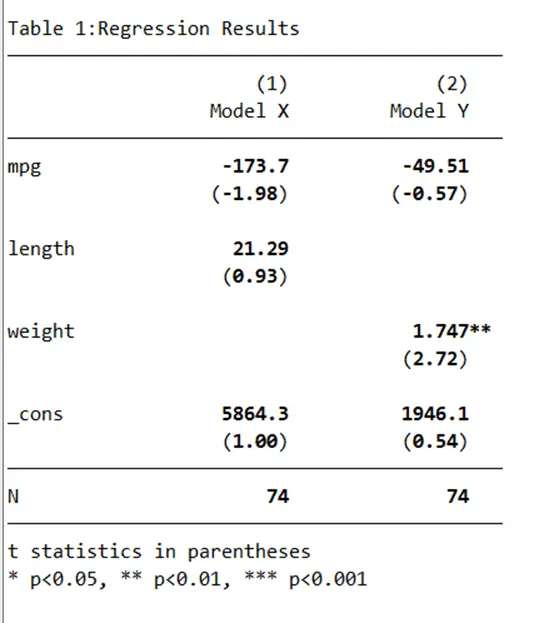
Moreover, “esttab” command can help in making custom titles too. We can use the “mtitles”, called the Model Titles, option along with our esttab command to customize titles on the columns. Along these lines, a command
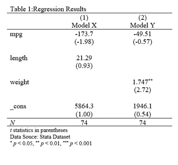
esttab, mtitles(“Model X” “Model Y”)
will show up like this,
Also, a command
esttab , mtitles("Model X" "Model Y") title("Table 1:Regression Results")would generate the title of the Table as well, as shown below,
Notes can be added with another command,
esttab , mtitles("Model X" "Model Y") title("Table 1:Regression Results") addnote("Data Souce: Stata Dataset")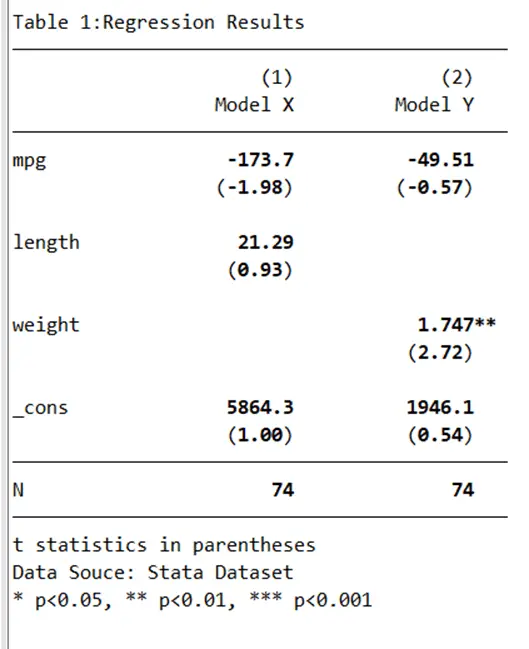
Remember, whenever you feel that a table is ready to be exported, you can always add “using results2.rtf” after your esttab command to export them in MS Word. Thus, the above derived results can be exported as such
esttab using results2.rtf, mtitles("Model X" "Model Y") title("Table 1:Regression Results") addnote("Data Souce: Stata Dataset")Your MS Word file, titled “results2” would show your table as follows,
The titles of the MS Word and MS Excel files can also be changed depending on your preferences. You can change them by changing the titles in the commands.
Replace an Existing Result With a New One:
Now, if you want to replace an existing file result with a new one, you are in the right place. First, let us alter some results with the command
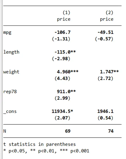
eststo length: regress price mpg length weight rep78
You would see the following results:

This action would replace the previous results stored with “length” to these results. Once you execute the
esttab
Command, this action will clearly show in the column corresponding to “length” that the previous results are replaced.
Regression by Group:
Let us do some regression by group. First, let us open the categoric variable that highlights whether the car is produced domestically or is foreign. You can open it through “Data Editor”. The column of this variable would look like this,
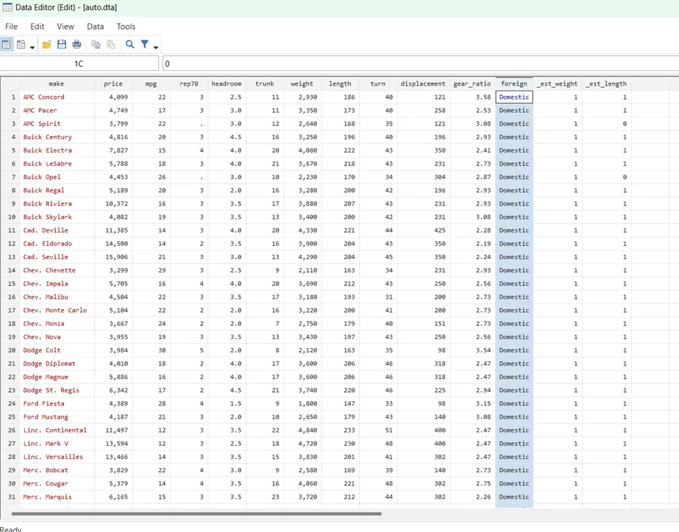
Our objective is to establish distinct regression models for each category: one for domestic cars and another for foreign cars. To achieve this, we adopt a structured approach. We use a command,
by foreign: eststo: reg price weight mpg
By executing this command, you can see the following,
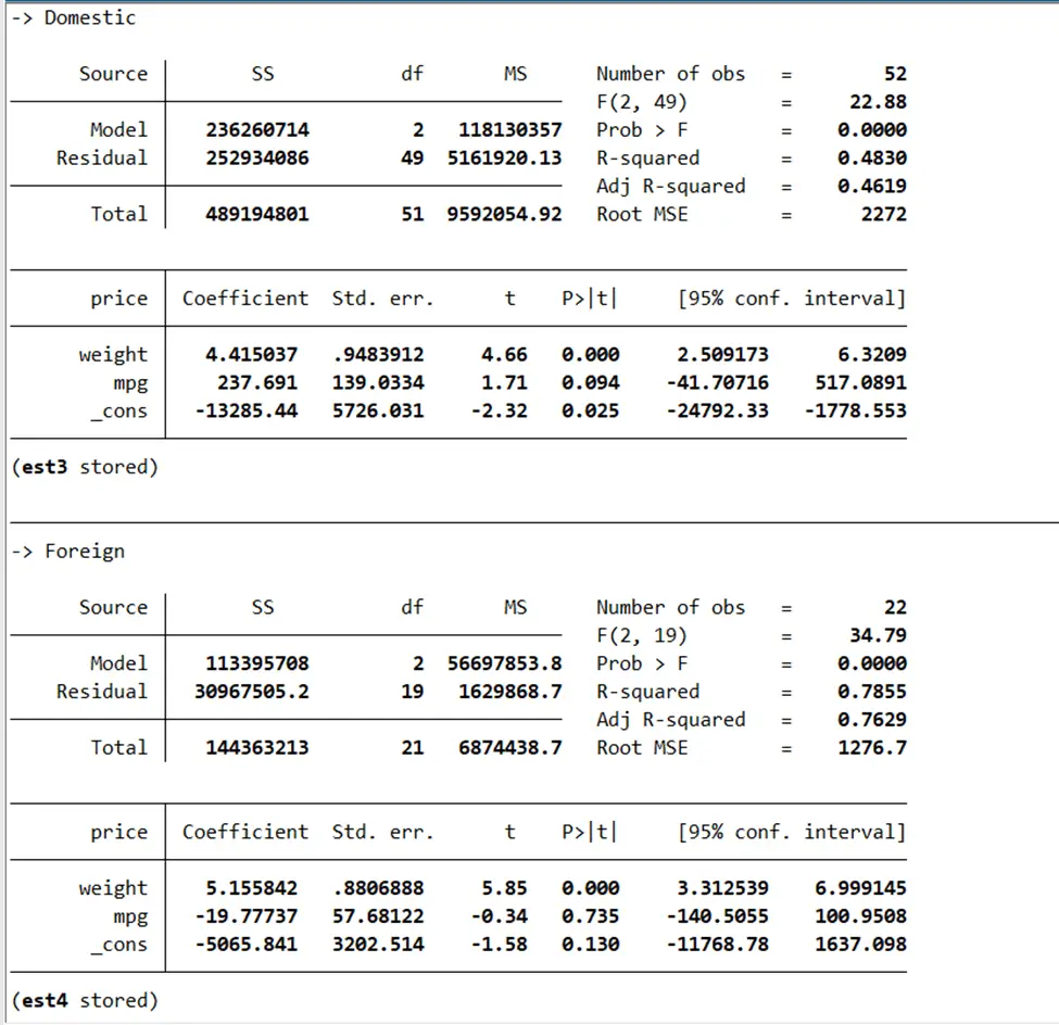
Firstly, we label the categorical variable as “Production Origin,” with values denoting either “Domestic” or “Foreign.” This categorical variable serves as a crucial factor in our analysis. To create separate regressions for each category, we employ a technique using the ESTIMATE (est) and STORE (sto) commands.
The
eststo label nodepvar
command allows us to store the results of each regression in separate columns named “length”, “Model 2”, “Domestic” and “Foreign”, as shown in the illustration below,
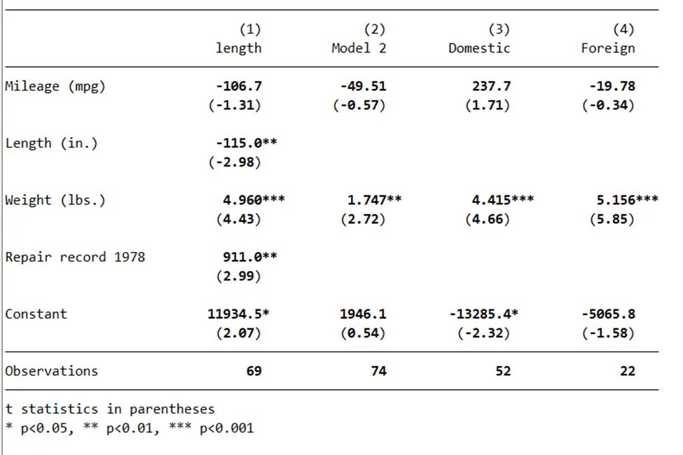
It’s important to note that throughout this process, we leverage the “label” and “no dependent variables” attributes to efficiently manage and distinguish between dependent variables and results. These labels offer clarity and insight into the specific variables used in the regressions and the outcomes associated with each regression category.
Options with esttab Command:
Jumping to the options related to “esttab” command, let us quickly revise that it can be used to export the data too. Upon visiting your directory by the command,
eststo dir
You can glance at your stored results quickly. From here you can choose the data you want to export.
The command,
esttab
Will show all the results like this,
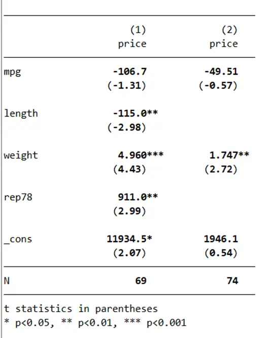
To export just the results stored by the name of length and weight , your command should be
esttab length weight
which will be executed as such,
To remove the parenthesis from the t-stats, the following command can help,
esttab length weight, noparen
Your result will show up without parenthesis.
Brackets can be applied to the t-stats through this command,
esttab length weight, brackets
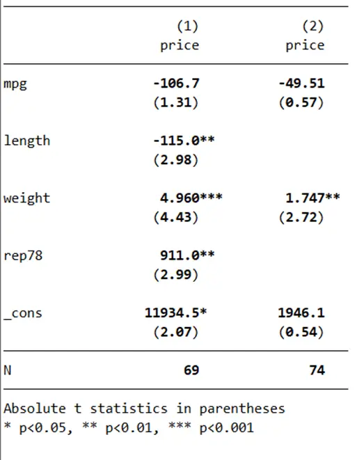
To convert t-stats into absolute form, the command
esttab length weight, abs
is required. The following illustrations shows the result,
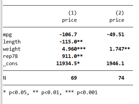
If you want to remove the t-test completely, you can use the following command,
esttab length weight, not
and your result will not show t-stats i.e.
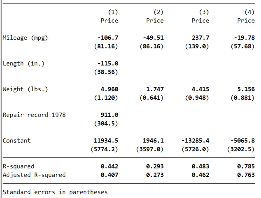
If you want the wide format, the command
esttab length weight, wide
Will help to visualize all statistics that one require including the coefficients, the t-test or standard errors. An example of the wide format with t-test is given below,
To have standard errors instead od t-tests, you can use the following command
esttab , se nostar r2 noobs label ar2
Although the command looks difficult, we can break it down to understand it better. By “se” we mean standard error, by “nostar” we mean that we do not need the Asterisk, or star, or * in our result. By “r2” we are clarifying that we can have r2 . By “noobs” we are explaining that we do not need observations, by “label” we mean that we are using labels instead of variable names and “ar2” is the adjusted r2 . If the command is let to work its magic, we are left with this,
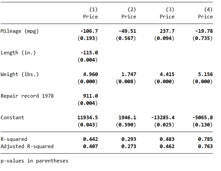
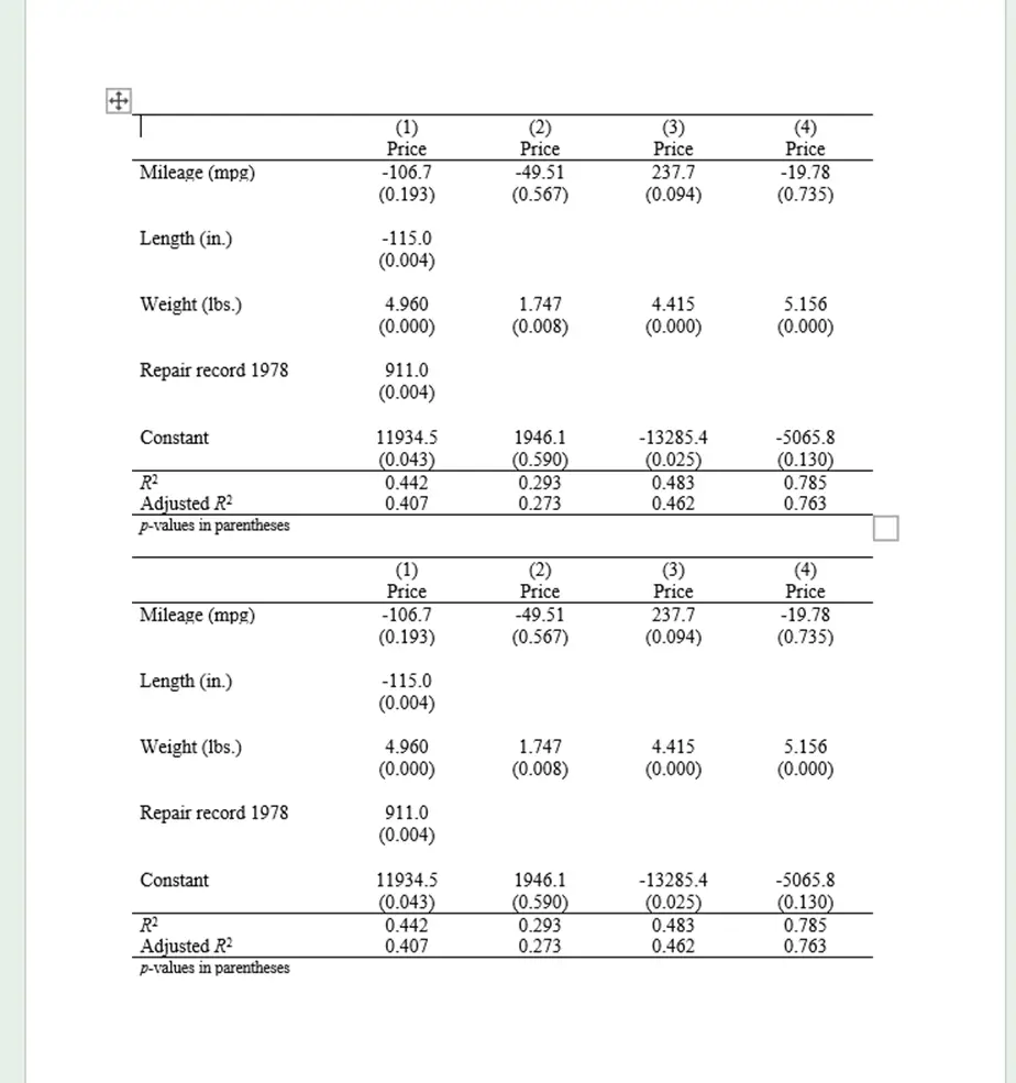
To have p-value in parenthesis instead of standard error, the command would be repeated but with a slight change,
esttab , p nostar r2 noobs label ar2
The Decimal points can be changed too! By Running this command, you can increase the number of digits after the decimal points,
esttab , b(2)
As shown above, the decimal points are increased. Along with beta, this command can be done on all kind of statistics including standard errors, p-value and confidence intervals and the t-value (e.g. se() p() ci() t()). For each stat, the command would change minutely to fit the specific stat.
You can thus save, replace and append the files. To refresh how replacing and appending works, we can quickly go through two commands,
esttab using results.rtf, p nostar r2 noobs label ar2 replace
would replace the previous data in the Word Document titled “results” while this command,
esttab using results.rtf, p nostar r2 noobs label ar2 append
would append or add to the available data in the Word Document titled “results”, as shown in the illustration below,
Thus, the “esttab” command be tailored to display specific outcomes, such as adjusted R-squared values or standardized coefficients. Decimal points can be adjusted to improve the precision of results.
By mastering the art of storing, customizing, and exporting statistical analysis results, you gain the prowess to present your insights with impact and clarity. Happy Learning!