
It is often a hassle to convert analysis tables created in Stata into professionally formatted tables that are acceptable for research publications. This problem is eased by a user-written command called asdoc in Stata which allows publication style output to be produced in Microsoft Word (the command cannot output tables to any other format currently). This command is also able to output summary statistics, correlation tables and frequency distributions, though in this article we keep our focus on outputting regression tables.
To begin our guide, we first load Stata’s inbuilt dataset through;
sysuse auto, clear
The syntax of asdoc is much simpler than outreg or estout commands. All we do is add the prefix asdoc to any command we wish to output the result of.
[bysort: varname:] asdoc Stata_command, [command_options asdoc_options]
The first part of the syntax above indicates that any categorical variable we may wish to sort our command on will be added through bysort first, just like it always is. This part can obviously be omitted if you don’t have to categorise your regressions/summary statistics on any variable.
The second part is simply an addition of the asdoc command, followed by any regression/summary statistic/correlation command you wish to run.
Options are treated just like they always are i.e followed by a comma after the main command. These options will include both the main command options (e.g. robust for a regression) and the asdoc options.
asdoc can output regression tables in three different formats:
- Full regression table
- Nested regression table
- Wide regression table
This article covers the full and nested regression tables. (The wide regression tables will be covered in another article).
Full Regression Table
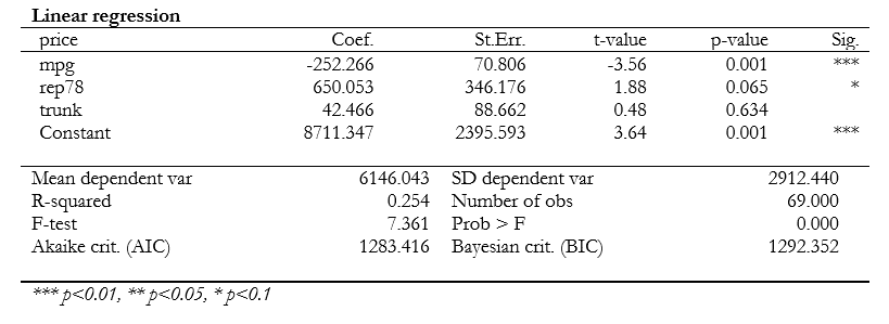
Following the syntax above, we run the following simple OLS regression:
asdoc regress price mpg rep78

This outputs a table that is slightly different from what we see in academic publications, but is a very comprehensive and detailed table that we can save and share with our coauthors. This table can then always be consulted for full results and comparisons with other regression outputs.
If we run another regression, its output table will also be added to the file which holds the results from the previous regression.
asdoc regress price mpg rep78 trunk
Removing Confidence Intervals
The column that reports confidence intervals can be removed using the noci option.
asdoc regress price mpg rep78 trunk, noci
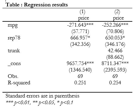
Nested Regression Table
Nested regression tables are the most frequently reported form of regression output that we see in research papers. To report these, we add an option of nested (or nest) as an option in our command.
asdoc regress price mpg rep78, nested save(newfile) replace

There are two other options in the command above. The save(filename) option is used to specify the name of the Word file which we want our output to be stored in. The replace option replaces any previous file that exists by the same name with a file with the new regression results.
Important Note: Typically when writing options in front of commands in Stata, we do not need to add a space between the comma and the option. This command however requires a space between the comma and the option that proceeds it.
Adding a New Column To an Existing Regression Table
To add a column to an existing regression table, we add the append option to the asdoc command:
asdoc regress price mpg rep78 trunk, nested save(newfile) append
Remember to specify the same file name as the previously created file (or whichever file you need your column added to), otherwise a new file will be created.
[embedyt] https://www.youtube.com/watch?v=ppHMXheyOqw[/embedyt]Specifying Decimal Places
In order to restrict the decimal places that are displayed in the output table, one can employ the dec() option where the number of decimal places we need is entered in the parenthesis.
asdoc regress price mpg rep78, nested save(newfile) replace dec(2) asdoc regress price mpg rep78 trunk, nested save(newfile) append dec(2)

The output of both regressions will be displayed correct to two decimal places now.
Changing Column Titles
Columns in the regression table will be titled with the name of the dependent variable by default. If we want to, for example, title our columns as ‘Model1’ and ‘Model2’, we use the option of cnames() with the desired column title written in the parenthesis.
asdoc regress price mpg rep78, nested save(newfile) replace dec(2) cnames(Model1) asdoc regress price mpg rep78 trunk, nested save(newfile) append dec(2) cnames(Model2)
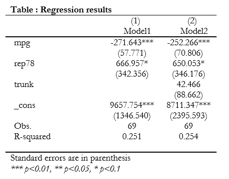
We can also change the font size of the column titles by modifying the cnames() option by adding a backslash followed by ‘fs’ and the fontsize (all without spaces) before the column title in the parenthesis. This is better understood by seeing the option written:
asdoc regress price mpg rep78, nested save(newfile) replace dec(2) cnames(\fs25 Model1)
The above command will output Model 1’s regression column that has a title of font size 25.
Related Book: Data Management Using Stata by Michael N. Mitchell
Table Title
It is also useful (and recommended) to give a title to the entire table that shows our regressions’ results. This can be achieved simply through the title() option where the parenthesis will hold the title that we wish to give our table.
asdoc regress price mpg rep78, nested save(newfile) replace dec(2) cnames(Model1) title(Regression Analysis)
This adds the title of ‘Regression Analysis’ to the table.
If we do not want any title, we modify the title() option by writing a back slash in the parenthesis:
asdoc regress price mpg rep78, nested save(newfile) replace dec(2) cnames(Model1) title(\)
Reporting T-Statistics Instead of Standard Errors
If we want t-statistics instead of standard errors reported under the coefficients, we add the option rep(t).
asdoc regress price mpg rep78 trunk, nested save(newfile) dec(3) cnames(Model3) rep(t) replace
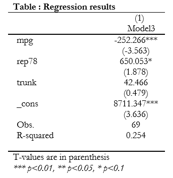
Note that this option can only be used with the replace or reset option.
Reporting Variable Labels Instead of Variable Names
Due to variable naming restrictions in Stata, variable names are often not very descriptive of the data they represent. For example, for anyone unfamiliar with the 1978 Automobile data, ‘rep78’ might not make much sense in terms of what it means. In such cases, we have the option of replacing variable names with variable labels in our regression table. This is achieved by using the label option in our command.
asdoc regress price mpg rep78 trunk, nested save(newfile) dec(3) cnames(Model3) rep(t) replace label
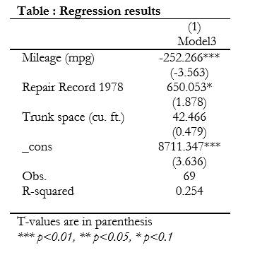
Now, in place of ‘rep78’, we see its label ‘Repair Record 1978’ which is much more descriptive and easier to understand.
Adding Rows to The Table
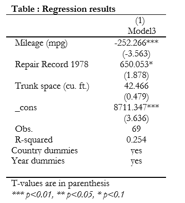
Usually we want to add additional rows to our regression tables that indicate the presence of certain dummies or time/cross-section fixed effects which are not otherwise reported. The option for the follows the following syntax:
add(column 1 text, column 2 text, column 1, text column2 text)
The first argument appears in the first column, while the second argument appears in front of it in the second column. The third argument moves to the next row and appears again in the first column, followed by its corresponding text in the second column.
asdoc regress price mpg rep78 trunk, nested save(newfile) dec(3) cnames(Model3) rep(t) replace label add(Country Dummies, Yes, Year Dummies, Yes)
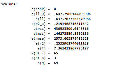
Reporting Additional Statistics
We can report additional statistics in the regression table using the stat() option. The parenthesis will be populated with the macro variable of whichever statistic we want to add. Macro variables that contain statistics can be checked by entering the following command right after a regression or summary command:
ereturn list
Alternatively, we can also browse through the documentation for the regress command which describes the statistics stored in each macro under the ‘Stored results’ section. This document can be opened by executing:
help regress
Similarly following command will report the adjusted R-squared and the F-statistic.
asdoc regress price mpg rep78 trunk, nested save(newfile) dec(3) cnames(Model3) rep(t) replace label add(Country Dummies, Yes, Year Dummies, Yes) stat(r2_a, F)\
Omitting or Retaining Variables
You can choose which variables to keep or drop in the results table through the keep() and drop() options respectively. drop() omits any variable that we specify in the parenthesis. keep() displays only the variables that we write in the parenthesis.
asdoc regress price mpg rep78 trunk, nested replace drop(mpg)
The command above omits the results of the ‘mpg’ variable from being reported. This variable will still be included in the regression analysis; its output just won’t be reported.
asdoc regress price mpg rep78 trunk, nested replace keep(rep78 trunk)
This command displays regression results only for the ‘rep78’ and ‘trunk’ variables. Here as well, ‘mpg’ will be included in the regression analysis, but output for only ‘rep78’ and ‘trunk’ will be reported.
Formatting Font Size and Font Style
By default, the output table generated through asdoc is formatted with a font style called Garamond in size 12. The options fs() and font() let us change the font size and font style respectively.
asdoc regress price mpg rep78 trunk, nested replace fs(12) font(Arial)
Through this command, our output table will have a font style of Arial in size 12.
The options of fhr() allows us to format the row header, while fhc() lets us format column headers. The parenthesis for each of these options need to be populated by rtf controls. These rtf controls are listed in detail in the help documentation of the asdoc command which can be accessed through:
help asdoc
There are many other options that allow us to align asdoc() with our purpose, all of which can be studied through the help documentation of the command.
option nested not allowed in Logit Model, any suggestions
Thank you for the video. Please, how do I connect with you. I am in the middle of data analysis. I need your assistance.
Please email me at info@TheDataHall.com