
In this article, we will go over the difference between R-Class and E-Class commands and how we can access information through them. Whenever we execute a command in Stata, it stores the results in one of these commands. It is very common to use these commands to extract and use the result they store in subsequent command for data analysis or summary.
Download Example FileTo get a comprehensive understanding of E-Class and R-Class commands, it is important for you to understand what scalars and matrices are and how they work in Stata.
Defining the Two Command Types
E-Class commands are estimation class commands. Any time you run a regression command that estimates some kind of parameters, the results get stored in this type of commands.
Other commands that return results like summary stats, test results, tabulation etc. come under the R-Class command type.
R-Class Commands
Whenever, we execute a command, its results will be stored in a scalar or a matrix. R-Class commands store the results in the ‘r’ scalar expressed as r().
Let’s use Stata’s built-in automobile dataset to illustrate how R-Class commands work. We will also summarize the ‘mpg’ variable.
sysuse auto.dta, clear summarize mpg
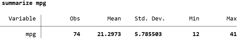
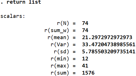
The statistics that the summarize command returns (and some more) are stored in predefined scalars by Stata. They can be checked by using the following command:
return list
Related Article: Local and Global Macros in Stata
This command returns the list of scalars and the corresponding statistics that are stored in them. For example. ‘r(N)’ stores the number of observations that the summarize command returned. We can display these scalars, or execute certain commands using them.
display r(max)
This displays the maximum value (41) of the ‘mpg’ variable that was summarized. More than displaying these values, these scalars are used more often in conducting other operations and analysis. If, for example, we want to create a variable called ‘maxvar’ that should contain the value stored in the ‘r(max)’ scalar, we can do the following:
gen maxvar = r(max)
In this case, this new variable will have the value of 41 for all observations.
We can also perform calculations using these scalars:
display r(max) - r(min)
This calculates the range of the variable that was summarized without us having to input the numbers on our own.
So, how do we know what scalar name corresponds to which statistic? One way to do it is what we described above, i.e. use the return list command and get a list of all the scalars that store a statistic. But some stats in this list are not entirely self-explanatory about what they are, nor are they displayed in the summary table. For example, it may not be immediately obvious what the scalar r(sum_w) intends to display. To obtain these details, simply open the help page for the summarize command using the command help summarize and scroll to the bottom. There will be comprehensive list of all the R-class scalars produced by the summarize command, and a description of what they represent. r(sum_w) shows us the sum of weights.
A more manual approach is to compare the values returned by the summary table with the values in the scalar list (list produced using return list command). We can see that the value of 12 here corresponds to r(min) so it is clear that this scalar holds the minimum value of the variable summarized. This approach is however prone to errors since it is possible that more than one summary statistic holds the same value. In this case, r(N) and r(sum_w) have the same value of 74 even though they represent different statistics. It is best to refer to the descriptive list in the help section in this case.
Related Book: Data Management Using Stata by Michael N. Mitchell
R-Class Scalars and the Summary Detail
Another way to look at how R-Class scalars are used is through the summary detail command which entails adding an option to the summarize command:
summarize mpg, detail
Adding this option returns us a more detailed summary table that includes statistics like different percentiles, skewness, kurtosis, and the four smallest and largest values. The scalars that hold these values can be obtained through the same command as before:
return list
We can know that r(p50) stores the median value or r(skewness) stores the skewness value.
R-Class Scalars and the t-test
Let’s use the t-test command to determine whether the prices for foreign and domestic cars are same or not. The price is stored in the ‘price’ variable, while the ‘foreign’ variable is a binary indicator of whether a car is local (0) or not (1). To check whether the prices across these categories are statistically similar or not, we use the following command:
ttest price, by(foreign)
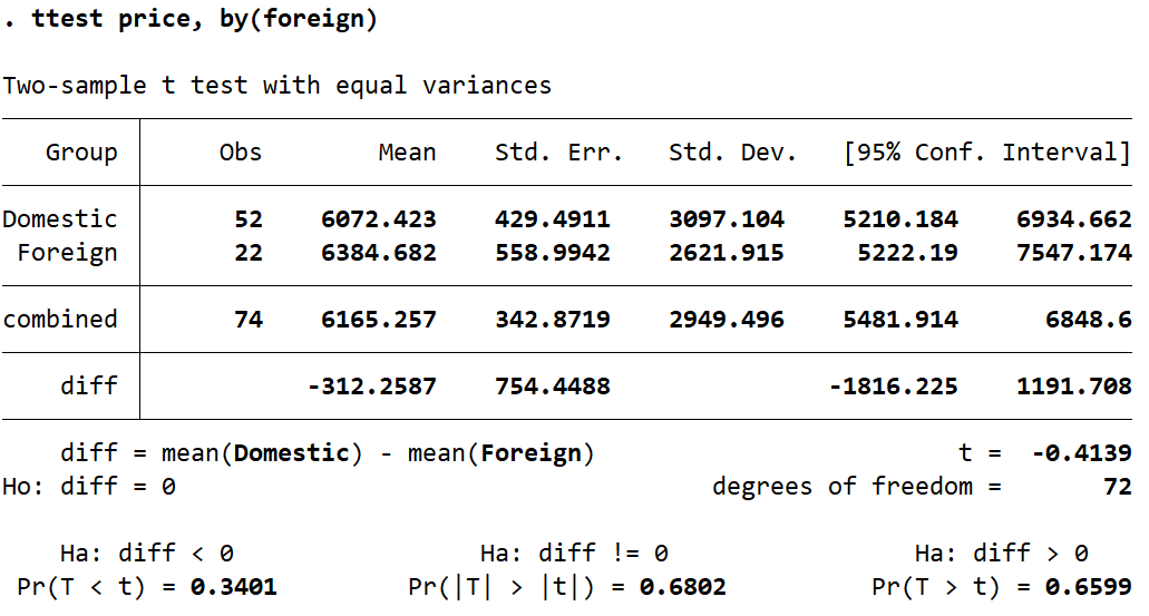
The table that we obtain shows us that the difference between the mean of the price of both categories is 312.26 (domestic cars being cheaper). To determine if this differences is statistically significant, we check the t-stat labelled simply ‘t’ in the table. In this case, the small t-stat of -0.4139 indicates that the difference is not statistically significant.
Let’s see what scalars are stored by Stata for this t-test.
return list
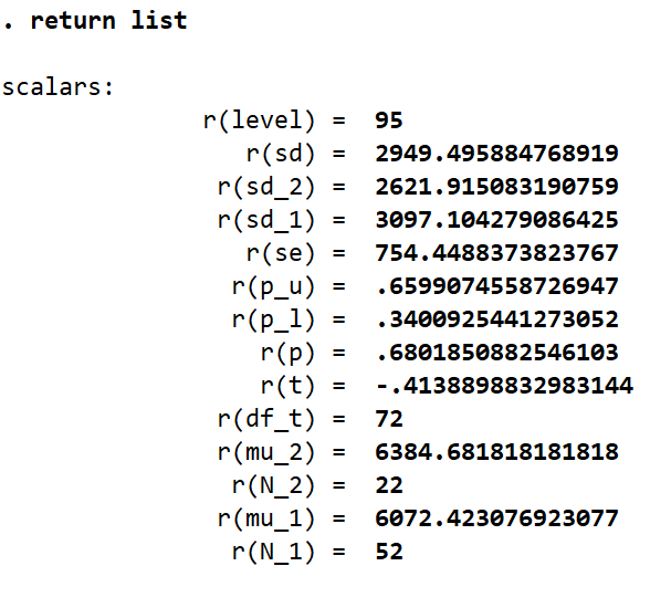
In the list of scalars that we get, it is interesting to note that there is no scalar that stores the difference in means (-312.25). This is because Stata does not store values that are a result of some calculations done on the produced statistics. In this case, the mean price values for both the categories are saved in their respective scalars. Their difference or the resultant t-stat is not saved in any scalar. This avoids redundancy as we can use the scalars for the standard error and the scalars for the means to calculate these two subsequent statistics. The difference in means can be calculated as follows:
display `r(mu_1)’ - `r(mu_2)’
This returns us the value of -312.25.
The t-stat can be calculated by replicating the scalars in the formula we typically use to calculate this statistic:
display (`r(mu_1)’ - `r(mu_2)’)/r(se)
This returns us the same value of -0.4139 displayed in the table.
E-Class Commands
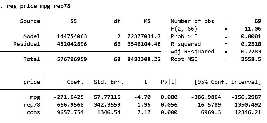
E-Class commands return us regression results where coefficients and relevant statistics are stored in scalars written as ‘e()’. Let’s execute a regression command:
reg price mpg rep78
In order to obtain the list of scalars that are created after such a regression command, we use:
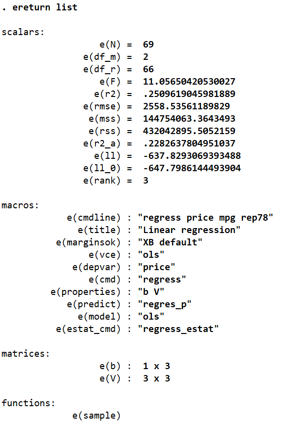
ereturn list
We get four categories of scalars in this list: scalars, macros, functions, and matrices.
Related Article: How to use Scalar and Matrix in Stata
Macros:
The macros simply store string values that indicate some features of the regression. Macros are covered in greater detail in a dedicated article.
Scalars:
As with R-Class commands, the list of scalars hold the values that are produced by the regression directly. This includes the number of observations, the degrees of freedom, F-stats, R-squared etc. We can again use these scalars to produce such statistics ourselves by writing them out in a formula form. R-squared, for example, can be calculated using the formula: explained sum of squares/total sum of squares. Remember that the denominator is a sum of the explained sum of squares, and the residual sum of squares.
In this case, the R-squared value can be obtained by using the scalars for these relevant statistics.
Using the help regress command, we can see that the explained sum of square, aka model sum of squares, is stored in the scalar e(mss), while the residual sum of squares is represented by the scalar e(rss). The R-squared value can then be obtained as follows:
scalar rsquare = e(mss) / (e(mss) + e(rss))
The scalar command stores the result of this formula in a scalar called ‘rsquare’. To display the result, we use the display command:
display rsquare
Functions:
The functions section stores the cases/observations that were used in the preceding regression. Stata’s regression command does not always use the complete sample available in its regression analysis since Stata makes use of what is called ‘casewise deletion’. This means that regressions are only executed for cases/observations where data for every variable is available. Therefore, if any observation includes a missing value for any variable involved in the regression, it will not be used.
.In the regression performed above, the top right part of the table shows that 69 observations were used even though the dataset has 74 observations. Through manual inspection, or suitable commands (e.g. codebook), we can see that five observations have a missing value for the variable ‘rep78’ which explains why the regression above had made use of only 69 values.
The function section comes in handy when, for example, you wish to report the summary statistics for the observations used in your regression. Such summary statistics can be obtained using:
summarize if e(sample) == 1
This will return a table of summary stats for only the 69 observations included in the regression.
Alternatively, you can also generate a variable that indicates whether an observation was a part of the regression or not:
gen sample = e(sample)
The new variable called ‘sample’ would take a value of 1 if the corresponding observation’s data was included in the regression, and 0 otherwise.
Matrices:
There were two matrices stored in Stata’s memory after the earlier regression was run:
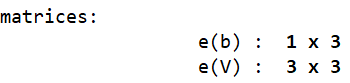
The first matrix, e(b), is a row vector of coefficients. Since this regression involved two covariates (independent variables), it stores the two corresponding coefficient and one intercept value.
The second matrix, e(V), is a square matrix of the variance and covariance of the covariates involved in the regression.
In order to see what a matrix stores, we run the command:
matrix list e(b)
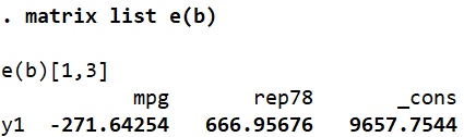
As explained before, this 1×3 matrix shows the corresponding coefficients for the two covariates (mpg and rep78) and the intercept term (_cons).
If we wished to retrieve only one specific value from the matrix, we can specify its position and Stata will display what that “location” in the matrix holds.
display e(b)[1,1]
This command asks Stata to display the value present in the first row and first column of matrix e(b). Note that there is no space between e(b) and [1,1]. This command returns us the value of -271.64.
If this specific value were to be stored in a scalar called bmpg, we would use a similar syntax in the following form:
scalar bmpg = e(b)[1,1]
Let’s now look at the variance-covariance matrix.
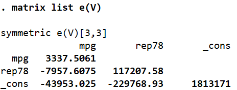
The diagonal terms are the variances of the variables while the other stats are the covariances between the corresponding variables.
Now, suppose we wanted to obtain the standard errors that the regression returned (in order to, e.g. manually calculate the t-stat). These statistics were not explicitly stored in any of the scalars that ereturn list provided us with. But we do know that the standard errors are simply the square root of the variance of a variable. We can display the standard error of a variable by using the square root function, sqrt, function in Stata.
display sqrt(e(V)[1,1])
As apparent, this command will display the square root of the value stored in the first row and first column of matrix e(V). In this case, this would be the standard error of the variable mpg – 57.77.
Values from both matrices can now be used to calculate and display the t-stat for a coefficient (formula: parameter estimate divided by its standard error). For the mpg coefficient, this can be attained by:
display e(b)[1,1] / sqrt(e(V)[1,1])
This returns us the value -4.70, which can also be confirmed through the regression table.
An issue that may come up in such a series of commands and calculations is the rearrangement of covariates in the regression commands. In this case, ‘mpg’ was the first covariate so we kept referring to the first row and first column of matrices. What if rep78 were typed in before mpg? The matric arrangement would alter accordingly as well.
An easier and more straightforward way to call upon regression specific stats is to use system variables called underscore variables. These are built-in variables with a preceding underscore sign that, in this particular case, can be used to refer to coefficient values of variables from the most recently run regression model. Here, this variable is _b.
display _b[mpg]
This command, for example, will return the beta coefficient for the mpg variable in the most recent regression.
display _b[_cons]
This command displays the intercept coefficient.
We can also use this approach to get an estimate for specific values of our covariates. What would the estimated price be if mpg equalled 20, and rep78 equalled 3? The following command would give us the answer:
display _b[_cons] + _b[mpg]*20 +_b[rep78]*3
The result suggests that a car with a mileage of 20mpg, and 3 repair records would be estimated to cost 6225.77.
We can also reference standard errors through such a notation. Instead of _b, we will use _se.
display _se[mpg]
We can also do the t-stat calculation using a combination of both underscore variables.
display _b[mpg] / _se[mpg]
Finally, there is one last matrix that is worth looking at in relation to the regression command. Instead of ereturn list, run the command return list.
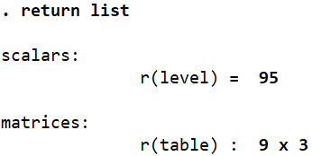
There is 9×3 matrix called r(table) that Stata also stores in its memory following a regression. To see what it stores, we run the matrix list command again:
matrix list r(table)
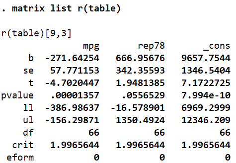
We can use the values for the beta coefficients, standard errors, t-stats and the other six statistics listed by referencing the correct position of a value. For example, the t-value of mpg can be reference as follows:
display r(table)[3,1]
This is genius