Panel data, also known as longitudinal data, involves collecting observations on multiple entities (such as firms, individuals, or countries) over multiple time periods. Researchers often use fixed effects, which can be in the form of time dummies or industry dummies, to account for various sources of data variation. In this article, we will test the significance of the time fixed effect in R and explore whether they should be incorporated.
Here we will conduct tests (using R Studio) to assess the importance of these time-fixed effect or year-fixed effect dummies in our analysis and to represent their results.
Panel Data Time Fixed Effect
In R we start every project with the installing and loading of required libraries. For the Time Fixed Effect, we need the following libraries.
Use the following command to install the required libraries:
install.packages (c("plm", "tidyverse", "stargazer"))To load them use these commands:
library(plm) library(lmtest) library(stargazer)
These libraries are essential for examining data, reading data, performing panel data regression, and generating simple regression summary tables. For more details about the use of different codes and their function related to Panel data models, see the article on Panel Data
Load panel data from a csv file
To load the data, we use the following command as an example for year fixed effect in R:
data <- read.csv("nlswork.csv")To examine the data use:
View(data)

The above figure is a snapshot of our data.
Panel Data Time Fixed Effects
model_tfe <- plm(ln_wage ~ hours + ttl_exp + factor(year) , data = data, model = "within", effect = "individual")
the above command runs the Time-fixed effects panel data model. The [factor(year)] indicates the time dummy or time-specific factors in R.
To see the results of the executed model we use:
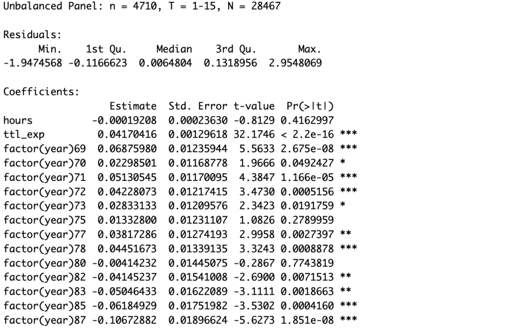
summary(model_tfe)

As shown in the above figure, here in this model, the time variable is included. To test whether it’s reasonable to include it or not, we can perform a Wald test, which compares the F-statistic with the p-value of two models: one with time-fixed effects and one without year dummies.
To Perform an F-Test to Test the Significance of Fixed Effects
We use a model without year-fixed effects (as we did here) and perform an F-test to compare it with the fixed effects model:
The command for making a model without time fixed effects is hereunder (note: the time fixed effect model(model_tfe) is already created):
model_no_tfe <- plm(ln_wage ~ hours + ttl_exp , data = data, model = "within", effect = "individual")
To execute F-test
f_test <- pFtest(model_tfe, model_no_tfe)
To see the results use:
print(f_test)

The results will indicate whether time-fixed effects significantly improve the model, typically by comparing p-values.
Here (see the above figure) the p-value (which is less than 0.05) states that adding fixed effects significantly improves the model. The F-test is a statistical test used to compare the goodness of fit between two models, typically a simpler model and a more complex model. It evaluates whether the more complex model significantly improves the model’s explanatory power compared to the simpler model.
Generating a Simple Regression Summary using Stargazer
In Panel data, time dummies are introduced for different years which makes it harder for a reader to read the results of a model. To overcome this and present the regression results neatly follow the following steps/commands.
models_list <- list(model_tfe, model_no_tfe) independent_variables <- c("hours", "ttl_exp") model_labels <- c(paste("Fixed Effects (", paste(independent_variables, collapse = ", "), ")", sep = "")) stargazer(models_list, title = "Fixed Effects Panel Data Regression", align = TRUE, style = "default", type = "text", column.labels = model_labels)
The above commands help us in making a simple summary table that includes model labels and independent variable names and important test statistics. Otherwise, it shows a bulk of dummy variables (see the following figure)

Perform Random Effects Regression (Optional)
If we aim to perform random effects regression and test the significance of a specific factor, we can use similar commands. This time, we chose ‘idcode’ as our fixed effect (any variable can be used in our pdata frame). It helps control for entity-specific factors across the entire dataset. To
model_tre <- plm(ln_wage ~ hours + ttl_exp + factor(idcode) , data = data, model = "random", effect = "individual") model_no_tre <- plm(ln_wage ~ hours + ttl_exp , data = data, model = "random", effect = "individual") fr_test <- pFtest(model_tre, model_no_tre) print(fr_test)
We can conduct fixed effects and random effects panel data regression in R and assess the significance of time fixed effects in our dataset, using this tutorial. Additionally, we can generate regression summary tables with or without fixed effects for further analysis. To know more about panel data models stay tuned to thedatahall.com
