
Researchers and analysts consistently endeavour to derive significant insights to inform decision-making and policy development in an era of abundant data. Panel data analysis is a robust methodology that offers insights into longitudinal patterns and reveals valuable information within intricate datasets. This article explores panel data analysis, explaining its fundamental nature and various applications.
Definition of Panel Data
Panel data /Pooled data/ Longitudinal data is the data that contains both time and space dimensions. In other words, it can be explained as the data structure combining multiple cross-sectional and time series periods. A cross-section of data is gathered at any given time, including information from various entities. These cross-sectional data are taken at different points in time and added together. This makes a panel data that includes information from many different times and places or individual. Panel data, as a result, offers a rich and potent resource for investigating how particular entities change over time and how they interact with different variables. This allows researchers to explore intricate relationships and find hidden patterns that are difficult to find using cross-sectional or time-series data alone.
Example of Panel Data
Here is an example of the panel data:
| Firm ID | Year | Net Income | Total Assets |
| 1 | 2020 | 2.2 M | 10.4 M |
| 1 | 2021 | 1.9 M | 8 M |
| 1 | 2022 | 3 M | 12 M |
| 2 | 2020 | 8 M | 25 M |
| 2 | 2021 | 7 M | 24 M |
| 2 | 2022 | 9 M | 22 M |
The dataset provided meets the criteria for panel data because it includes details on multiple companies for three consecutive years (2020, 2021, and 2022). Data is provided for all three years for each firm. The dataset also contains two variables net income and total assets. The time-series dimension represents the three consecutive years (2020, 2021, and 2022), while the cross-sectional dimension represents the individual firms (Firm 1 and Firm 2). Hence, the cross-sectional and time-series dimensions form a panel data structure.
The below dataset comprises panel data at the country level. The data has multiple countries data for multiple times. Hence, this panel dataset integrates both cross-sectional and time-series dimensions.
| Country | Year | Population |
| USA | 2020 | xx M |
| USA | 2021 | xx M |
| USA | 2022 | xx M |
| UK | 2020 | xx M |
| UK | 2021 | xx M |
| UK | 2022 | xx M |
Another example is the blood pressure before and after taking medicine. The dataset includes multiple medicines (1 and 2) and blood pressure data before and after taking medications.
| Country | Year | Blood Pressure |
| Medicine 1 | Before | 130/90 |
| Medicine 1 | After | 120/80 |
| Medicine 2 | Before | 135/92 |
| Medicine 2 | After | 110/85 |
Balanced vs Unbalanced Panel Data
In panel data analysis, a balanced panel refers to a dataset where all entities, or observation units, are observed for an equal and consistent number of time periods. This implies that each element within the dataset possesses data accessible for every designated period, and no instances exist where any time period lacks data for any given element. The panel dataset exhibits balance as each entity is uniformly represented with an equal number of observations throughout the entire time period. Balanced panels are widely regarded as optimal for certain types of econometric analyses due to their ability to facilitate direct comparisons and mitigate concerns pertaining to the absence of data for entities or time periods.
An example of the balanced panel data is given below:
| Firm ID | Year | Net Income | Total Assets |
| 1 | 2020 | 2.2 M | 10.4 M |
| 1 | 2021 | 1.9 M | 8 M |
| 1 | 2022 | 3 M | 12 M |
| 2 | 2020 | 8 M | 25 M |
| 2 | 2021 | 7 M | 24 M |
| 2 | 2022 | 9 M | 22 M |
In this example, firms 1 and 2 have data available for all three years (2020, 2021 and 2022), making it a balanced panel data.
An unbalanced panel is a dataset with missing observations for one or more entities over various periods. Certain entities may possess complete data for all time periods, whereas others may exhibit gaps in their data for specific years. Unbalanced panel data is when data is missing for particular time periods due to various factors. The presence of unbalanced panels can present specific challenges in data analysis due to the potential impact of missing data on model estimation and the introduction of potential biases.
An example of the unbalanced panel data is given below:
| Firm ID | Year | Net Income | Total Assets |
| 1 | 2020 | 2.2 M | 10.4 M |
| 1 | 2021 | 1.9 M | 8 M |
| 1 | 2022 | 3 M | 12 M |
| 2 | 2021 | 8 M | 25 M |
| 2 | 2023 | 9 M | 22 M |
In this example, firm 1 has data for three years from 2020 to 2022, while Firm 2 has data for two years, 2021 and 2023. This makes it unbalanced panel data.
To summarize, balanced data refers to a scenario where entities are present in all time periods, while unbalanced data refers to a situation where entities have varying numbers of time periods.
Regressor
In panel data analysis or econometrics, the term “regressor” pertains to an independent or predictive variable employed within a regression model. The regressor can be of three types:
1. Varying Regressor: The varying regressor is the one that varies or changes over time and across different entities such as net income, production etc.
2. Time Invariant Regressor: The time-invariant regressor is the one that remains constant through the time for each entity, such as gender, race, geographical location of the firm etc.
3. Individual Invariant Regressor: An individual invariant regressor is that one that remains constant over the entities but varies over time, such as inflation. For instance, we have firm-level data of USA firms. All these firms will face the same inflation for a specific year. However, it changes from year to year.
Panel Data Analysis
There are multiple techniques under the panel data analysis, as shown below image:
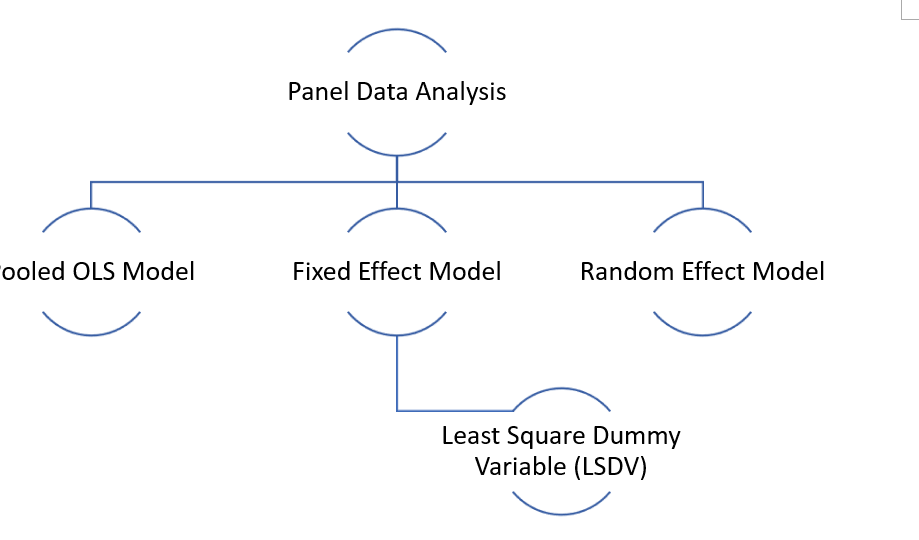
Other than that, there are some other techniques too that include:
- Between Estimate (BE)
- Within group Estimate (WG)
- First difference Estimate (FD)
This article will only focus on the pooled OLS, fixed, and random effect models.
Pooled OLS Model
Pooled Ordinary Least Squares (OLS) is a widely employed statistical regression model that estimates the association between a dependent variable and one or more independent variables. The term “pooled” denotes the characteristic of the data utilized in this model, wherein it originates from diverse sources or groups yet is amalgamated for analysis. The pooling of data is conducted based on the underlying assumption that the relationship between the variables remains constant across all the groups.
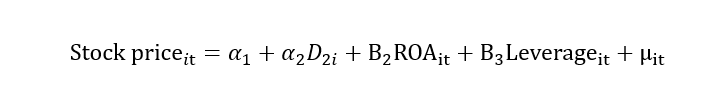
For example, we have data for stock prices, return on assets (ROA) and leverage. The stock price is a dependent variable, while return on assets and leverage is independent variables. The regression model is given below:
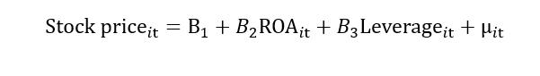
I represent cross-section data in the above model, and t represents time series data. This “it” represents that we have data on stock price, return on assets and leverage for different firms for different time periods. Hence, the “it” subscript represents that the data is a panel, the “i” subscript represents data in a cross-section, and the “t” subscript represents data in time series.
In pooled OLS model, we assume that the firm does not have individual effects, which means the regression coefficient is the same for each firm.
Limitation of the Pooled OLS model
Some unobserved factors also impact the dependent variable, such as two-time invariant factors, firm culture, and organizational culture, which can also affect the stock price. As we can’t observe these factors, we call them individual heterogeneity, unobserved heterogeneity and unobserved firm-specific characters that would impact the stock price. These factors affect go into the error term.
If there is a correlation between these error terms and the independent variable, the endogeneity problem arises. This problem provides biased estimates. Also, according to the regression assumption, there should not be an endogeneity problem.
Let’s explain it with the help of the example:
Suppose the organizational culture (time-invariant variable) is an unobserved factor that affects the stock price.

Let’s donate this OC as “αi”. Here, “i” show that this variable is time-invariant as it does not change with time.

All the time-invariant unobserved factor effect will go into the “αi”. Both αi and μit will form the composite error term “νit”. This composite error term includes the impact of individual heterogeneity and random error. Now, if this νit correlates with the ROA, then it leads to the problem of endogeneity.
Fixed Effect Model
This limitation with the Pooled OLS model can be resolved by using the fixed effect model. Another name for the fixed effect model is the least square dummy variable (LSDV). We know that αi contains the unobserved/individual heterogeneity. Let’s break this αi into multiple dummies for each firm. Suppose we have four firms; therefore, we will create four dummies as shown below:

When we add these dummies into the model, the impact of the unobserved factor will be excluded from the error term. In other words, this unobserved/individual heterogeneity (αi)will be removed from the composite error term (νit), and we will be left with random error (μit). In this way, the problem of heterogeneity also mitigates. We can also write it as:

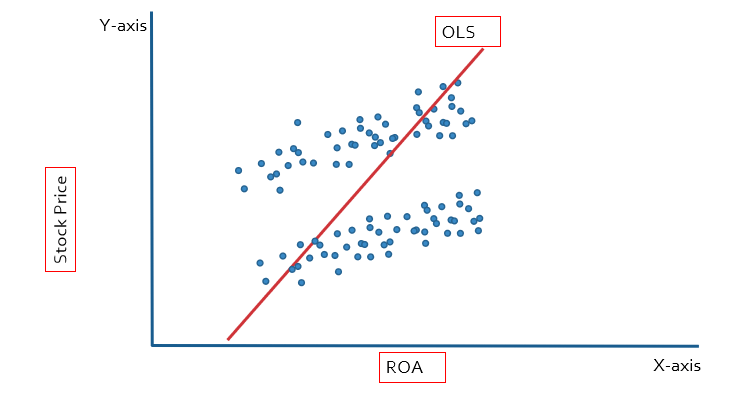
We used the dummy variable to deal with the heterogeneity problem, which is why this method is known as the least square dummy variable (LSDV). Let’s explain it with the help of the graph. The stock price is the dependent variable, so it is plotted on the y-axis, and ROA is the independent variable, so it is plotted on the x-axis. In the case of OLS, we will get the single slope and intercept for the multiple companies, leading to biased results.
In the case of fixed effect we will get multiple intercepts because we have created multiple dummies. Each firm is going to have a different intercept, as shown below figure:
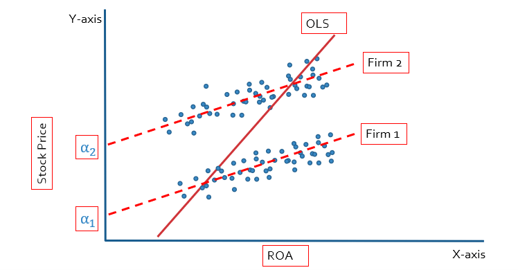
If we have more than two firms, the regression equation with dummies will look like this:

Limitation of Fixed Effect Model
- The degree of freedom will be less as we have included the dummy variable in the model, reducing the degree of freedom.
- Due to the dummies within the model, the problem of multicollinearity can arise.
- Lastly, the fixed effect can not be used with time-invariant regressors such as gender, race, or ethnicity.
Time/Industry/Country Fixed Effect
Fixed effect means introducing a dummy for years, industries and countries. In panel data analysis, researchers often use fixed effects to control specific factors that could influence the relationships between variables of interest. Time/Industry/Country fixed effects are a comprehensive approach that simultaneously considers time-specific, industry-specific, and country-specific effects. By including dummy variables for each time, industry, and country, the model accounts for variations related to these factors, allowing researchers to focus on the core relationships they aim to study. This method ensures that unobserved time, industry, or country-related shocks or trends are properly accounted for, resulting in more accurate and reliable estimates. However, it is crucial to be mindful of the potential challenges of multicollinearity and data requirements when employing multiple fixed effects in the analysis.
Random Effect Model
The random effects model is another statistical and econometrics method for evaluating panel data. It is a linear regression model that considers the data’s between-entity (group) and within-entity (individual) variation. When there is reason to suppose that each entity in the panel has distinct qualities that are not directly observed but are thought to be randomly distributed, the random effects model is used. The basic assumption of the random effects model is that individual effects, sometimes referred to as random effects or unobserved heterogeneity, are unrelated to the independent variables. Unlike the fixed effects model, which allows these individual-specific effects to be associated with the independent variables.
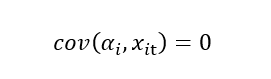
If there is no correlation of error term with the independent variable, then we use the random effect model.
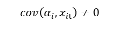
And if there is a correlation of error terms with the independent variable, then we use the fixed effect model.
Note: Fixed effect model can also be used if there is no correlation between the error term and the independent variable.
Should we use OLS, Fixed or Random Effect Model?
Before knowing which model to use, it is necessary to see if there is a panel effect. We use the “Breusch Pagan Test” to test this.The hypothesis of the Breusch Pagan Test is:
Ho: No panel effect
H1: Panel effect exists.
If the p-value> 0.05, then the null hypothesis will be accepted. This means that no panel effect exists. So, in that case, will use the OLS model. But if the p-value < 0.05, the null hypothesis will be rejected, and the alternative hypothesis will be accepted, which means that the panel effect exists. So, in that case, will use the Fixed or Random Effect Model.
After this, the Hausman test will decide whether we will use the Fixed or Random Effect Model. The hypothesis of the Hausman test is:
Ho: Error is not corrected with the explanatory variable (Random Effect)
H1: Error is corrected with the explanatory variable (Fixed Effect)
If the p-value> 0.05, we will accept the null hypothesis and use the random effect model. But if the p-value < 0.05, we will reject the null hypothesis while accepting the alternative hypothesis and use the fixed effect model.
Thank you for this. I have done statistics on point-in-time data but not panel data. This was a good introduction, with more detail if it’s needed.