
In the previous article, we discussed the theoretical aspect of the panel data analysis, including the basic knowledge and limitation of the OLS, Fixed, and Random Effect Models. This article will demonstrate the application of various statistical models using Stata. Along with that, we will also look into the Breusch Pagan test and Hausman Test.
We will use the national longitudinal survey of young women’s dataset. The data is the panel. The dataset can be accessed by using the below syntax:
Download Example Filewebuse nlswork, clear
The number of observations in this dataset are around 28000. The sample size is extremely large, so we will first limit the dataset to 500 observations by using the below command:
keep in 1/500
Pooled OLS Model
Pooled Ordinary Least Squares (OLS) is a widely employed statistical regression model that estimates the association between a dependent variable and one or more independent variables. The command is given below for the OLS model.
regress ln_wage hours ttl_exp
regress is the command, ln_wage is the dependent variable, and hours and ttl_exp are the independent variables. On running the above command, you will get the below results:
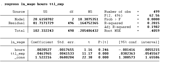
The p-value> 0.05 of the hours means that hours do not significantly influence the ln_wage, whereas the p-value < 0.05 of the ttl_exp means that ttl_exp has a significant influence on the ln_wage. The R square value of the model is 0.2015. According to this value, there is a 20.15% variation in the dependent variable due to the independent variables, while the remaining variation is due to some external factors.
Fixed Effect Model
In a fixed-effect model, individual-specific effects are treated as fixed constants. These individual-specific effects are time-invariant and capture unobservable characteristics that differ across entities but remain constant over time.
We will perform the fixed effect model manually and use the built-in STATA command to better understand. Note: It is not recommended to use the manual method of the fixed effect model. We have done manual method in this article to provide an understanding of the fixed effect model. Buildin Stata command is recommended as it is easy to use and saves time.
Manual Method of Fixed Effect Model
We discussed in our previous article that the fixed effect model contains dummies of different cross sections. In this dataset, these cross sections are represented by variable idcode (unique id of the individual). So, we will create the dummy for each id or idcode. For that, we will use the tabulate to generate the dummies of idcode. The command is given below:
tabulate idcode, generate(dummy)
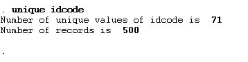
tabulate is the command, and idcode is the variable name. generate in the above command will create multiple dummies. This command will generate 71 dummy variables because our sample includes 71 unique ids or individual data. Use the below command to know how many cross-sections we have in our dataset of 500 observations.
unique idcode
Then we will run the below command to get fixed effect model results:
regress ln_wage hours ttl_exp dummy1-dummy71
regress is the command, ln_wage is the dependent variable, hours and ttl_exp are the independent variable, and dummy1-dummy71 are the 71 dummies we have created for each individual or idcode. The results are given below:
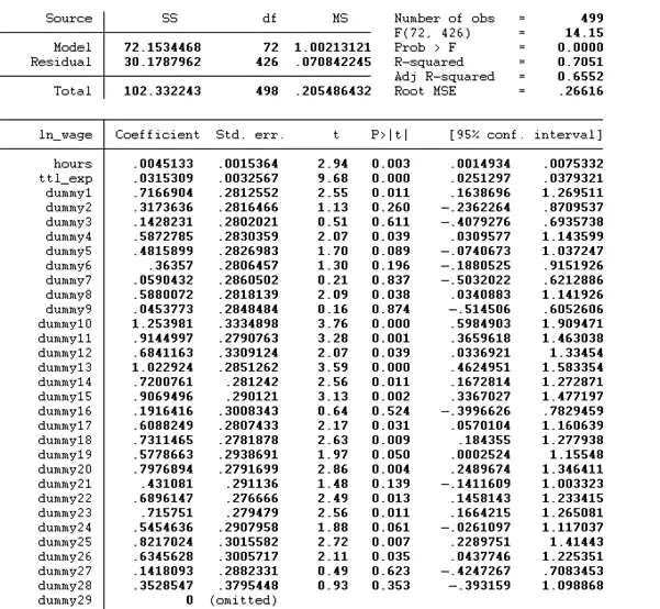
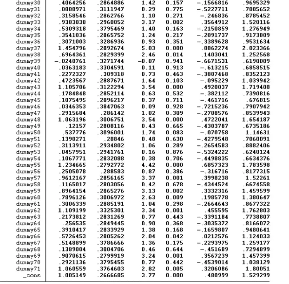
The dummy 29 is removed because if we have 71 dummies, we need to include 70, not all 71 dummies, within the model. As we include all 71 dummies, so STATA omitted itself. To overcome this issue, instead of adding all the dummies from dummy1-dummy71, we will exclude dummy1 from the model, as shown below. Note: this will not affect the results.
regress ln_wage hours ttl_exp dummy2-dummy71
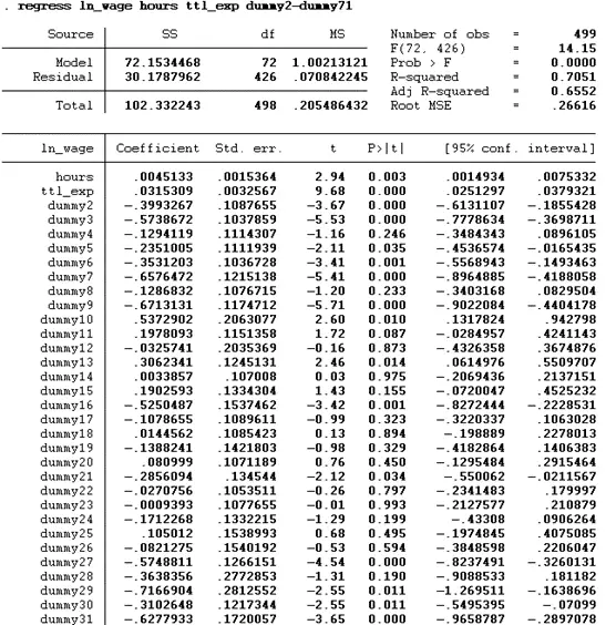
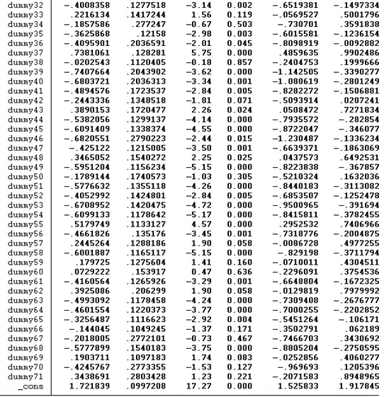
According to the above findings, the p-value of both hour and ttl_exp is below 0.05, indicating that both significantly influence the dependent variable ln_wage. The R square value of the model is 0.7051. According to this value, there is a 70.51% variation in the dependent variable due to the independent variables, while the remaining variation is due to some external factors.
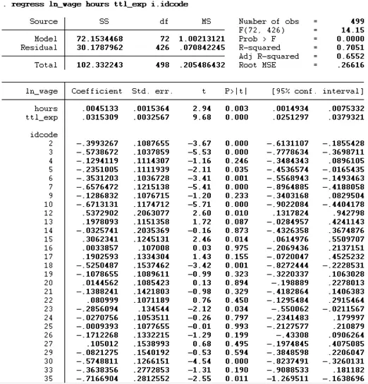
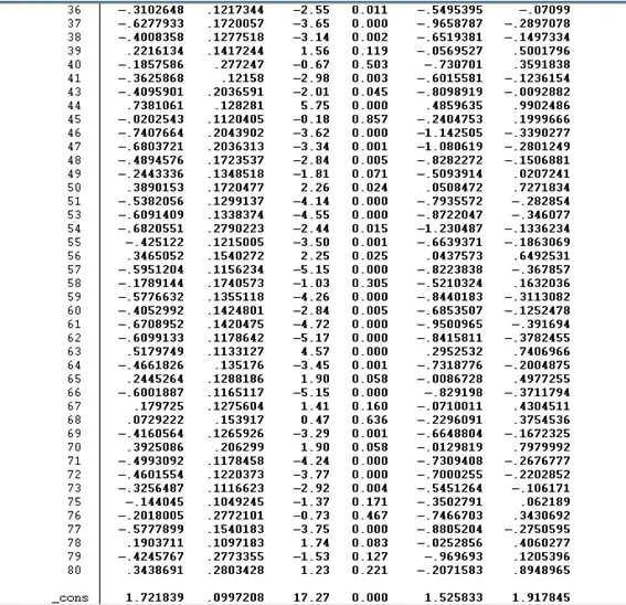
Another method to perform the above test is using the “i” and the idcode. This “i” will tell Stata that idcode is a categorical variable, and we want to see the impact of all these categories individually. This method will not generate a dummy but will provide similar results.
Now we will use built-in the Stata command xtreg. Before using the xtreg command, we must tell Stata that our data is the panel. This can be done by using the below command:
xtset idcode year
xtset is the command, idcode is the cross-section variable, and year is the time series variable.
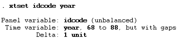
The data is unbalanced, which means that data is missing for time periods due to various factors. Sometimes, the cross-section variable is in string format, so in that case, it is a must that this cross-section data should be converted into numerical using the encode command. The command for the fixed effect model is given below:
xtreg ln_wage hours ttl_exp,fe
xtreg is the command, ln_wage is the dependent variable, and hours and ttl_exp are the independent variables. The fe after the comma is the function that represents the model we want to use is the fixed effect model.
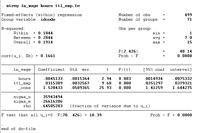
According to the above findings, the p-value of both hour and ttl_exp is below 0.05, indicating that both significantly influence the dependent variable ln_wage. The results remained the same as the manual method of the fixed effect model.
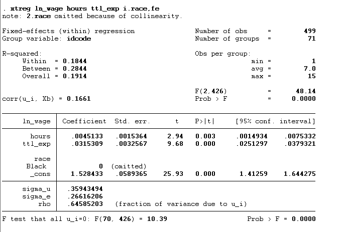
Remember, in the last article, we discussed that fixed effect could not be used with a time-invariant variable, so if we include the time-invariant variable in our model like below. It will omit that variable from the model. In the below command, “race” is a time-invariant variable.
xtreg ln_wage hours ttl_exp i.race,fe
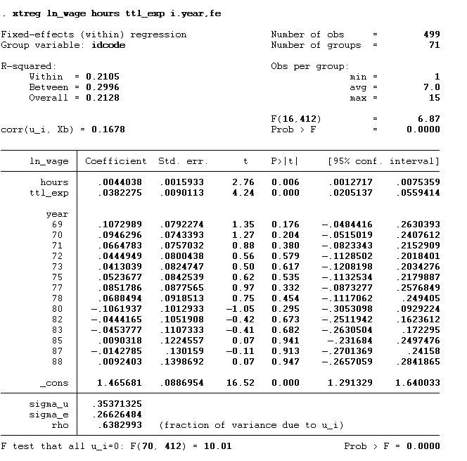
We can include year fixed effect in our model by using the below command:
xtreg ln_wage hours ttl_exp i.year,fe
Random Effect Model
In a random-effects model, individual-specific effects are considered random variables. These random effects are assumed to be uncorrelated with the independent variables, making them uncorrelated with the error term. For the random effect model, we use the same fixed effect model command; the only difference is we will replace the fe function with the re function. re tells that we want to use a random effect model.
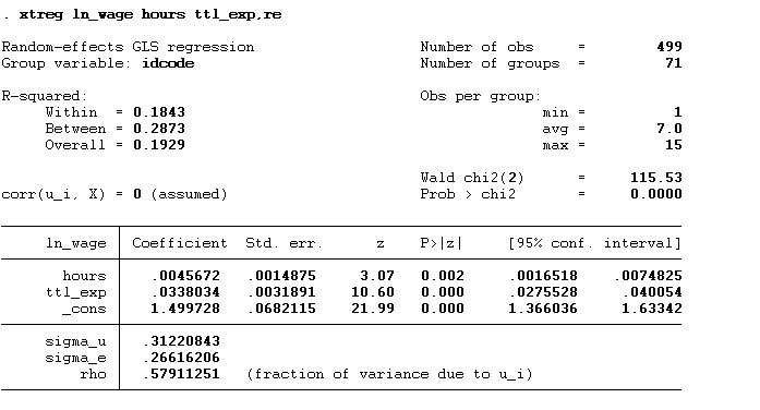
xtreg ln_wage hours ttl_exp,re
Breusch Panel Test
In our previous article, we discussed the “Breusch Pagan Test” used to test whether to use pooled OLS or random/fixed effect, i.e. is there a panel effect? We also discussed the hypotheses that are given below:
Ho: No panel effect
H1: Panel effect exists.
If the p-value is > 0.05, then pooled OLS is preferred
If the p-value is <= 0.05, then use the Hausman test to decide between a fixed or random effect model
For the Breusch Pagan Test, we will first run the model. Suppose we run the random effect model using the below command:
xtreg ln_wage hours ttl_exp,re
then we will run the below command to get Breusch Pagan Test:
xttest0
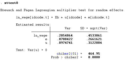
The p-value is less than 0.05; hence alternative hypothesis is accepted. This means the panel effect exists, so we must run the Hausman test to decide between a fixed or random effect model.
The hypothesis of the Hausman test is:
H0: Random effect is an appropriate model.
Ha: Fixed effect is an appropriate model
If the p-value is less than 0.05, then fixed effect is the appropriate model; otherwise use the Random effect model
There are five steps in the Hausman test:
Step 1: Run fixed effect model
We will run the fixed effect model using the below command:
xtreg ln_wage hours ttl_exp,fe
Step 2: Store the estimates
Then we will store the fixed effect model findings using the below command:
estimates store fixed
The finding will be saved with the name “fixed”.
Step 3: Run Random effect model
Thirdly, we will run a random effect model using the below command:
xtreg ln_wage hours ttl_exp,re
Step 4: Store the estimates
And then store the findings of the random effect model:
estimates store random
The finding will be saved with the name “random”.
Step 5: Run the hausman test
Lastly, we will run the Hausman test as shown below:
hausman fixed random
Hausman is the command, and fixed and random are the store results of fixed and random effect models.
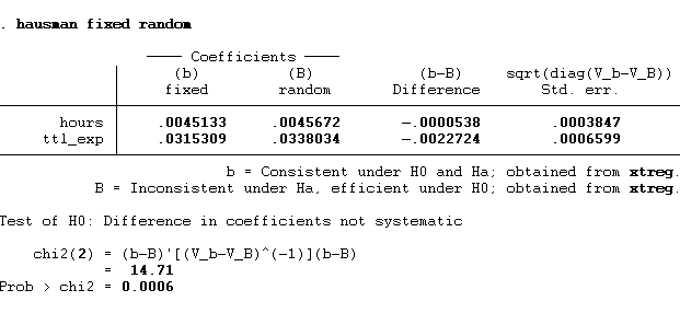
The p value < 0.05 therefore, we have enough evidence to reject the null hypothesis and accept alternative hypothesis which states fixed effect is an appropriate model.