
In the previous 2 articles we discussed the theoretical and practical implications of the Pooled OLS, Fixed Effect and Random Effect Models. This article will discuss the significance of dummy variables such as time or industry dummies in our panel data. We will use the same dataset we used in the previous article. The data can be accessed by using the below command:
Download Example Filewebuse nlswork, clear
The data is a panel containing the data for multiple individuals over multiple time periods. First of we are including the time dummy variable in the model. The command is given below:
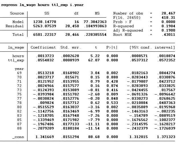
regress ln_wage hours ttl_exp i.year
regress is the command, ln_wage is the dependent variable, hours and ttl_exp are the independent variables, and year is the time variable. This “i” with the year tells Stata that year is a categorical variable, and we want to see the impact of all years individually. On running the below command, you will get the following results:
Wald Test
To test whether we should include this year’s (time) effect model, we need to run the Wald test. Wald tests to test the joint significance of the year dummy (time dummy). The hypothesis of the Wald test is also stated below:
Ho: Time fixed effect does not exist
Ho: Time fixed effect does exist
If the p-value is greater than 0.05, then the time-fixed effect does not exist and If the p-value is less than 0.05, then year dummies are jointly significant, and the time-fixed effect exists. The command for the Wald test is given below:
Note: Before executing this test, it is must that regression should be run.
testparm i.year
testparm is the command for Wald Test.
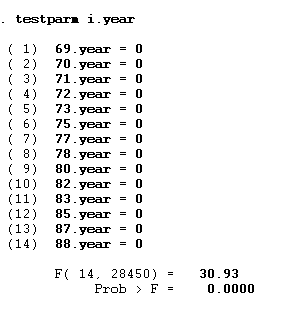
The p-value is less than 0.05, which provides evidence to reject the null hypothesis and accept the alternative hypothesis suggesting that year dummies are jointly significant and a time-fixed effect exists. The Wald test can also be performed for the fixed and random effect models.
Fixed Effect Model
First, we need to run the fixed effect model by using the below command:
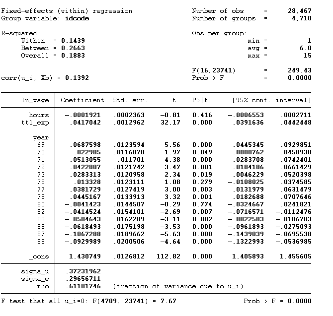
xtreg ln_wage hours ttl_exp i.year,fe
Then we will execute the Wald test command:
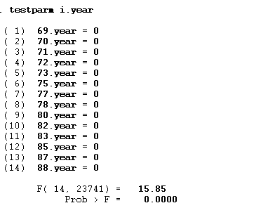
testparm i.year
Random Effect Model
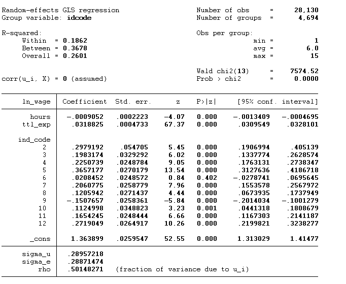
We will perform a similar step for the random effect model. First, we will run the random effect model command. Using the time effect is not a must; we can also use an industry dummy. In the random effect model, we are using an industry dummy. The command is given below:
xtreg ln_wage hours ttl_exp i.ind_code,re
Then Wald test command,
testparm i.ind_code
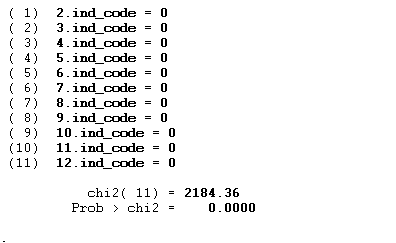
The p-value < 0.05 indicates that the industry effect exists.
Export Results
Researchers and analysts can easily export their Stata analysis results, graphs, or tables for later use or to share with others. Stata’s flexibility and adaptability come from its multiple exporting choices for findings. In this section, we will export Stata’s fixed effect or random effect results into the word format. Note: the method to export the fixed and random effect results is the same.
Firstly, we will run the fixed effect model using the same command as above:
xtreg ln_wage hours ttl_exp i.year,fe
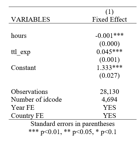
We are considering the year-fixed effect. After getting the fixed effect results, we will execute the below command:
outreg2 using results, word replace dec(3) title(Fixed Effect) add text(Year FE, YE)
outreg2 is the command to export the results into the Word file. Then we will use the using option that specifies the filename and path of the output file where the regression results will be saved. After using it, we will write the file name we want to save with. The word option specifies that the output will be in Microsoft Word format. If the file named in the using option already exists, Stata will overwrite it when you instruct it to do so with the replace option. If the file already exists, Stata will give an error if this replace option is not specified. The output’s precision can be tweaked with the dec option. In this scenario, the number of digits after the decimal point is set to 3. The title option creates a unique heading for the table or output. The export table will have a header reading “Fixed Effect” in this case. Users can customize their output by adding text with the add text option. The output will include “Year FE” and “YE” in this scenario.
We can add multiple fixed effects in the model as shown in the below command:
xtreg ln_wage hours ttl_exp i.year i.ind_code,fe
We will use the same command we used before to export the results. However, only the append option and addtext option will change.
outreg2 using results, word append dec(3) ctitle(Fixed Effect) addtext(Year FE, YES, Industry FE, YES)
The append option instructs Stata to append the output to the specified file if it already exists. If the file does not exist, it will be created. This is useful when adding results or tables to an existing file without overwriting the existing content. In this case, the add text option includes two additional labels in the output. The labels “Year FE” and “Industry FE” are now included in the output, both with the text “YES” as their values.
For instance, if the industry effect does not exist, then it would be wrong to write Yes. It should be No. So, in that case, we will change the command slightly, as shown below:
outreg2 using results, word append dec(3) title(Fixed Effect) addtext(Year FE, YES, Industry FE, No)
We will write the “No” after the industry effect. This “No” will replace the “Yes” in the table.
When reporting the results, you may not want to include every year and industry dummy variable since this could make the output very cluttered and hard to interpret (imagine a column for every year in your dataset, for example). The drop option can be used to execute these variables from the output table.
outreg2 using results, word replace dec(3) ctitle(Fixed Effect) addtext(Year FE, YES, Country FE, YES) drop(i.year i.ind_code)
By using the above command, the table will just report “Year FE: YES” and “Industry FE: YES”, which indicates that these variables have been controlled for in the analysis without reporting their specific effects.