In this article we will discuss how to perform correlation in R. We will discuss both the association between continuous variables and as well as association between categorical variables.
Correlation is a statistical term that describes a point to which two variables are associated or connected. It lets us figure out where and how variations in a specific factor affect variation in others. A correlation coefficient, which is a number with values ranging from -1 to 1, is often used to represent the relationship. Here are the different types of correlations:
| Positive Correlation | Negative Correlation | No Correlation |
| A correlation value close to +1 indicates a significant positive link. This means that as one factor rises, another one tends to follow suit. | A correlation coefficient close to -1 indicates a strong negative connection. This means that while one variable increases, the other tends to decrease. | When the correlation coefficient is near or equal to zero, there is hardly any linear relationship or no relationship between the two variables. |
| For example, there might be a correlation between the number of hours studying and test scores. | For example, there could be an adverse relationship between someone’s level of activity and their body weight. | For Example Student’s height has no relation to its studying hours or exam results. |
Pearson and Spearman correlation coefficients are two common methods for estimating correlation coefficients. They are used in various conditions based on the essentials of your data and the type of relationship you want to approach. We will exercise R’s built-in dataset “Iris” to understand. This dataset is generally used to test data analysis and categorization strategies. It includes lengths and widths of sepals and petals for three iris flower species. It has 150 observations and 5 variables. You can use the following code to load this dataset:
data(iris) head(iris)

Pearson’s correlation in R
Pearson correlation is a statistical method to distinguish the linear relationship between two variables that are both continuous. It is also known as Pearson’s r or commonly r. It regulates the strength and direction of a relationship between variables, assuming that the data is linearly connected and has a normal distribution. The syntax for Pearson’s correlation in R is
cor(x, y , method = c("pearson"))Here x and y are variables for which we will check correlation. The method is Pearson’s Correlation.
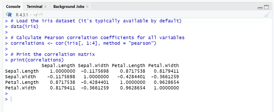
For example, if we want to check the correlation of all variables in iris data, we will use code:
# Calculate Pearson correlation coefficients for all variables correlations <- cor(iris[, 1:4], method = "pearson") # Print the correlation matrix in R print(correlations)

This correlation matrix exhibits the Pearson correlation coefficients among all pairs of variables in the “iris” dataset. We note that Petal Length and Sepal Length have a significant positive relationship (0.8718). It means that as Petal length increases Sepal’s length increases as well.
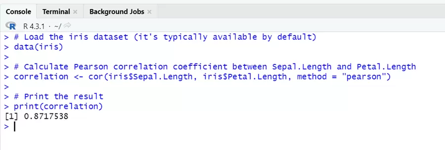
Similarly, if you want to check the correlation of 2 variables you can use the code:
data(iris) # Calculate Pearson correlation coefficient between Sepal.Length and Petal.Length correlation <- cor(iris$Sepal.Length, iris$Petal.Length, method = "pearson") # Print the result print(correlation)

Spearman Correlation in R (Spearman’s rank-order correlation):
The Spearman correlation coefficient is used to evaluate the strength and direction of a periodic (but not always linear) relationship between two variables. A periodic relationship is one in which the direction of the relationship remains consistent. It is especially useful when the data does not meet the normality criterion or the relationship between variables is not linear. Monotonicity of the relation of two variables is measured by this method.
Spearman’s correlation is determined using the data value’s ranks rather than their actual values. It initially ranks the data before computing the correlation between its ranks.
# Calculate Spearman rank correlation in R on the 'iris' dataset correlation <- cor(iris$Sepal.Length, iris$Petal.Length, method = "spearman") # Print the Spearman correlation coefficient in R print(correlation)

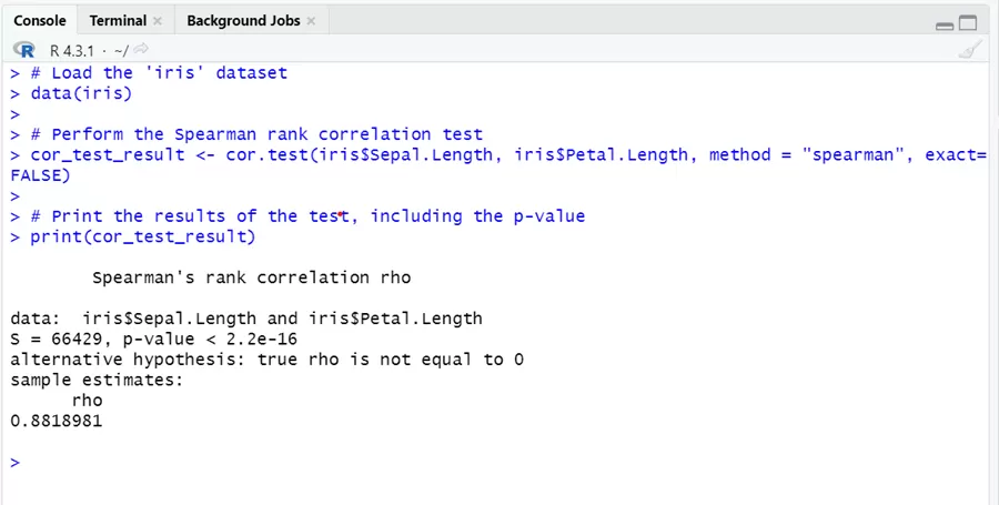
For the significance of this correlation, we can use the code below:
# Load the 'iris' dataset data(iris) # Perform the Spearman rank correlation test cor_test_result <- cor.test(iris$Sepal.Length, iris$Petal.Length, method = "spearman", exact= FALSE) # Print the results of the test, including the p-value print(cor_test_result)

The p-value (2.2e-16) is quite close to zero. A p-value less than the ordinary significance level of 0.05 indicates that the observed association is statistically significant in the sample. The extremely low p-value indicates a highly significant relationship, meaning that the observed relationship did not happen by chance.
If the data has ties (same observations), we can use Kendall tau’s approach, which is less affected by ties.
Here is the code:
# Calculate Kendall's Tau correlation <- cor.test(iris$Sepal.Length, iris$Petal.Length, method = "kendall") # Print the Kendall's Tau correlation coefficient print(correlation)

Kendall’s Tau correlation between ‘Sepal.Length’ and ‘Petal.Length’ is highly statistically significant (p-value 2.2e-16), showing a somewhat good relationship between these two variables.
Correlation of Categorical Variable
The most common application of correlation is to detect the strength and direction of a link between two continuous (numerical) variables. We cannot use correlation if any of the variables in the pair is categorical. We’ll start with the metrics. Correlation is more difficult to determine when working with categorical variables because simple correlation coefficients such as Pearson’s correlation or Spearman’s rank correlation are used for numerical data. Instead of correlation, methods designed for categorical data can be utilized. Let’s understand it with some examples.
There are three common approaches:
Tetrachoric Correlation:
Tetrachoric correlation is a method for determining the strength and direction of a link between two binary variables. The calculation of this correlation lies under the assumption of normality. It is a sort of point-biserial correlation. For example we are interested to check that whether there is any link between gender and favorite sport.
| Gender/Favourite Sport | Soccer | Basketball |
| Male | 30 | 20 |
| Female | 7 | 10 |
R code for this correlation is :
library(psych) #create 2x2 contingency table data = matrix(c(30,7,20,10), nrow=2) #view table data #calculate tetrachoric correlation tetrachoric(data)

The tetrachoric correlation in this scenario is 0.28. It indicates moderate positive correlation and mirror the degree and direction of the association between gender and favorite sport. A tetrachoric correlation of 0.28 indicates that persons of a given gender have a severe preference for a particular sport.
Polychoric Correlation
Polychoric correlation examines the relation between two or more ordinal categorical variables that rely on the assumption of continuous distribution.
Suppose we have a dataset of customer satisfaction and service quality. Customer Satisfaction is scaled as “Very Satisfied (1), Satisfied (2), Neutral (3), Dissatisfied (4) and Very dissatisfied (5)” and Service Quality is scaled as “Excellent (1), Good (2), Fair (3)”.
| Sr.no | Customer Satisfaction | Service Quality |
| 1 | 5 | 1 |
| 2 | 2 | 2 |
| 3 | 3 | 3 |
| 4 | 4 | 3 |
| 5 | 1 | 1 |
R code is :
library(polycor) # Define Ratings Customer_Satisfaction<-c(5,2,3,4,1) Service_Quality<-c(1,2,3,3,1) polychor(Customer_Satisfaction,Service_Quality)

In this example the polychoric correlation is roughly 0.1669. This result is close to zero, indicating that the link between “Customer_Satisfaction” and “Service_Quality” in the data is very weak or non-existing.
Cramer’s V
Cramer’s V is a substantive measure of significance for nominal or ordinal categorical variables. It measures the strength of correlation between two categorical variables rather ordinal or nominal by taking the dimensions of a contingency table into account. The Cramer’s V scale goes from 0 to 1 (perfect association). It is often used to measure the strength of connection in categorical data contingency tables. Chi-square tells us “Is there any relationship between dependent and independent variable” while Cramer’s V tell us how strong the relation is.
Assume you want to investigate the strength of relation between two categorical variables, “Gender” and “Favorite Sport,” and you’ve gathered the following information:
| Gender/Favourite Sport | Soccer | Basketball | Tennis | Swimming |
| Male | 30 | 20 | 20 | 30 |
| Female | 7 | 10 | 15 | 10 |
| Prefer not to say | 5 | 10 | 9 | 25 |
R code for Cramer v is
library(rcompanion) #create table data = matrix(c(30,7,5,20,10,10,20,15,9,30,10,25), nrow=2) #view table data #calculate Cramer's V cramerV(data)

Cramer’s V of 0.4551 is a relatively high figure. This indicates a moderate to strong relationship between the two categorical variables represented by the contingency table. It tells us that there is a relationship between the variables, but it does not explain why this relationship exists.
Listwise, Casewise, Pairwise Correlation
Correlations between variables can be calculated using a variety of approaches, including listwise, casewise, and pairwise correlation.
1. Listwise Correlation: In this method we exclude all rows/cases which have any missing value in any of the variables. Simply, a case which has missing value in any of the variable will be excluded from analysis for all the variables in data and analysis will be done on cases which have all the information.
2. Casewise Correlation: This method computes correlations for each pair of variables by taking into account only the cases (rows) in which both variables contain non-missing values. The cases which have non-missing value in the selected variables for correlation will be excluded from the data.
3. Pairwise Correlation: This method computes correlations for all pairs of variables and deals with missing values through pairwise deletion. In other words only that pair of case will remove in which there is missing value. If the same case has non-missing value in other variables, it will not be deleted.
Assume you have a dataframe named ‘df’ with several variables and wish to calculate the correlations between some of them. We’ll use three different approaches in this example. Here’s how to use the ‘cor()’ function to calculate each of these correlation approaches. In this example, we are generating random numbers for a sample data frame.
# Create a sample dataframe set.seed(123) df <- data.frame( Customer_Satisfaction = rnorm(100), # Represents customer satisfaction scores Product_Quality = rnorm(100), # Represents product quality ratings Sales_Performance = rnorm(100) # Represents sales team performance metrics ) # Add some missing values df$Customer_Satisfaction[c(5, 15, 25)] <- NA df$Product_Quality[c(10, 20, 30)] <- NA # Listwise Correlation (Complete Cases) listwise_corr <- cor(df, use = "complete.obs") print("Listwise Correlation:") print(listwise_corr) # Casewise Correlation casewise_corr <- cor(df, use = "pairwise.complete.obs") print("Casewise Correlation:") print(casewise_corr) # Pairwise Correlation pairwise_corr <- cor(df, use = "pairwise") print("Pairwise Correlation:") print(pairwise_corr) 
