In regression analysis, quantifiable data often steals the spotlight. Yet, there are instances where qualitative or categorical variables like gender, ethnicity, age groups, or even something as simple as car colours play a crucial role. How do we seamlessly integrate these categorical variables into our statistical models? Take, for example, a study examining how gender affects wages; how do we translate the categories “Male” and “Female” into a language our statistical model understands? The answer lies in creating dummy variables that act as numerical stand-ins for these categories. In this comprehensive article, we delve into the mechanics of dummy variable regression analysis, specifically focusing on handling single categorical variables. Along the way, we’ll explore the significance of margins and margin plots using a diverse dataset for hands-on illustration.
Download Example File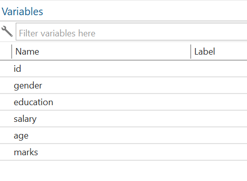
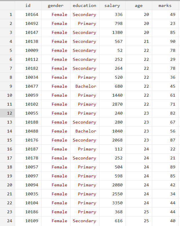
The dataset contains two categorical variables, gender (male and female) and education (Bachelor, Master, Primary, and Secondary), and three continuous variables, salary, age, and marks.
Generate Dummy Variables
In this article, we’ll explain the two main ways to create dummy variables, making it easy to choose the best method for your needs. One thing that we need to understand while working with the dummy variable is that if we have m categories, then there will be an m-1 dummy variable. A key point to remember is the “m-1 rule” for dummy variables: if you have ‘m’ categories in your qualitative variable, you will need ‘m-1’ dummy variables in your model. For instance, a variable with two categories would require only one dummy variable, whereas a variable with four categories would require three dummy variables.
Method 1: Manual Method to Deal with Dummies
In this first method, we will generate the dummy manually. The first step is to tabulate the variable and then generate multiple variables based on categories. The command for the tabulate, along with the generate option, is given below:
tabulate gender, generate(gender)
On execution of the above command, the two variables will be generated as shown in the below Figure:
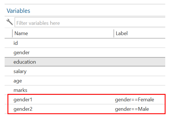
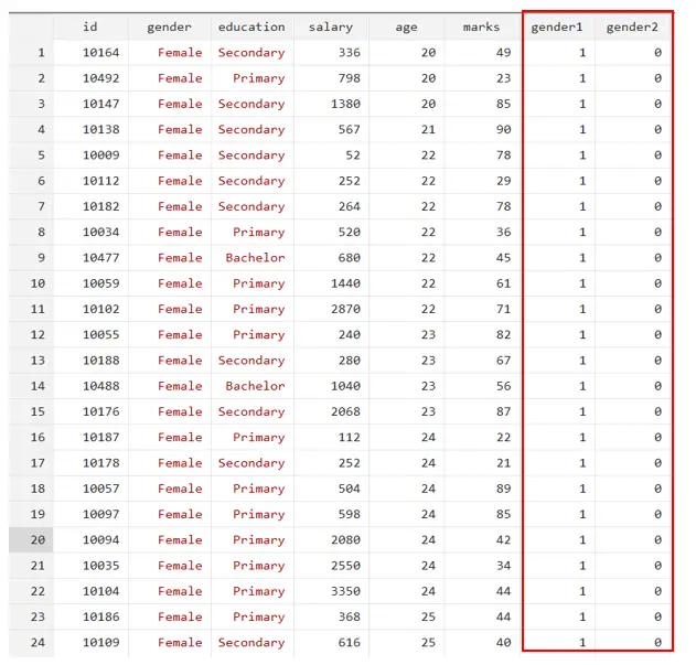
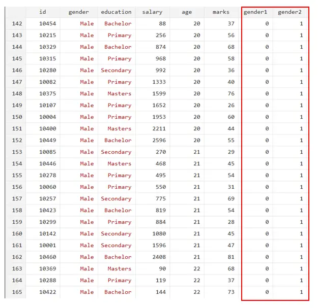
Gender1 represents female respondents, and gender 2 represents male respondents. You will see that gender1 has a value of 1 if the gender = female and 0 if it is male, as shown in the above Figure. Similarly, gender2 has a value of 1 if the gender is male and 0 if the gender is female.
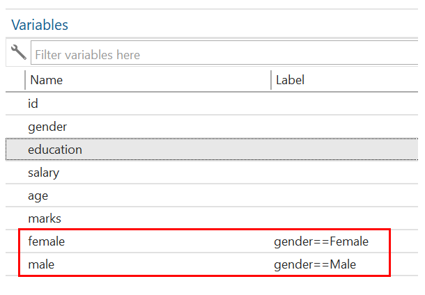
To make it easy to understand, we can rename the variables gender 1 = female and gender 2 = male by using the below commands:
rename gender1 female rename gender2 male
Now, we will run the regression with the male dummy using the below command:
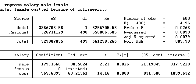
regress salary male
Here, we added only one dummy male, not a female. In this example, we’ve included only the male dummy variable, deliberately omitting the female one. Adding both would lead to dummy variable trap. If it’s essential to include all dummy categories in the model, one solution is to remove the constant term (also known as the alpha) to avoid this error. The result of the above command is given below:
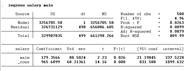
These results show that males significantly influence salary (p-value < 0.05). If the gender is male, their salaries will be 179.37 units (or dollars in this example) greater than the females. The calculation of the salary is shown below:
Salarymale = α + β1 (Male) + ε
Salarymale = 965.61 + 179.357 (Male)
Salarymale = 965.61 + 179.357 (1) = 1144.967
Salaryfemale = 965.61 + 179.357 (Female)
Salaryfemale = 965.61 + 179.357(0) = 965.61
You can notice the expected salary of the omitted category (female in this case) is shown by the constant term.
The error that we will get by adding both dummies to the model is also shown below in Figure:
We can also execute the above regress command with a female dummy variable instead of male. The command is given below:
regress salary female
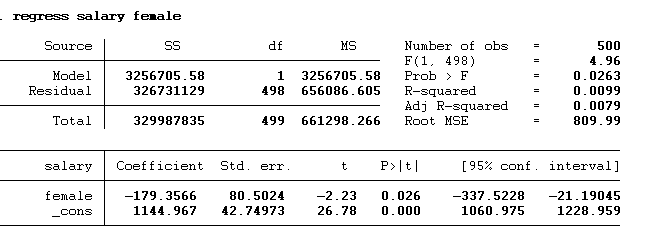
The p-value < 0.05 indicates that females have a significant influence on salary. The beta coefficient suggests the negative impact of females on salaries. Females earn 179.37 less than males. The final salary for both males and females will remain the same. However, the beta and the constant values will be different. So, whether you take one category as base category or another, the conclusion remains the same. The calculation is given below:
Salaryfemale = α + β1 (Female) + ε
Salaryfemale = 1144.967 – 179.357 (Female) + ε
Salaryfemale = 1144.967 – 179.357 (1) + ε = 965.61
Salarymale = α + β1 (Male) + ε
Salarymale = 1144.967 – 179.357 (0) + ε = 1144.967
Simple Method to Deal with Dummies
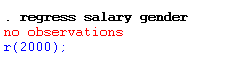
As we can see, gender is both a categorical and a string variable. So, if we run the regression using gender (string variable), we will get an error. The error is shown below:
If we add “i” (to tell Stata that gender is a categorical variable) with the gender and run the regression, we will again get the error. The error is given below:
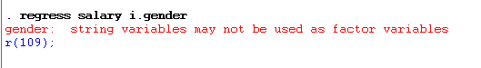
This error is because gender is the string variable. Therefore, we first need to convert the gender categorical variable into the numerical coding using the encode command with the generate option. The command is given below:
encode gender, generate(gender_e)
We will use this new encoded gender variable in the regression model. This encoded variable assigned 1 value to the female and 2 to the male. After encoding, the next step is to regress the dependent variable (salary) against the independent variable (gender). The regress command is given below:
regress salary i.gender_e
You can notice that we have used gender_e (the encoded variable) instead of the gender (which is the string variable. The results are shown below:
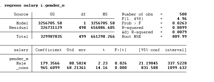
The results are the same; Males earn 179.357 times more than females. You will notice that the female category is omitted from the model. To see which category is omitted, we can use the all base levels option with the regression as shown in the below command:
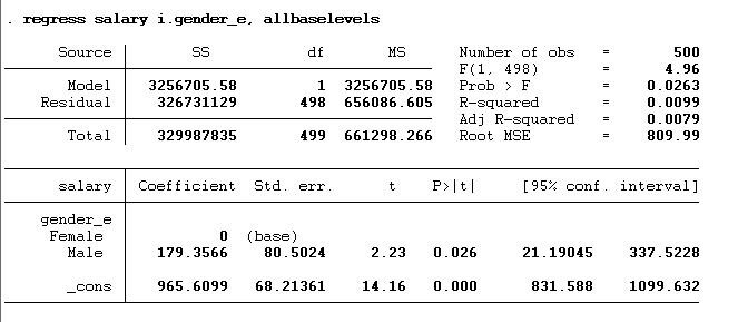
regress salary i.gender_e, allbaselevels
The results we will get from the execution of the command are given below:
Margin and Margin Plot:
When dealing with continuous and categorical predictors, it is common to be interested in how a continuous variable might interact with a categorical variable in predicting the response. The relationship between the continuous predictor and the response might not be the same at each level of the categorical variable, indicating an interaction effect. In statistical modelling, “margins” refer to the predicted values of the response variable at specific “typical” values of the predictors. For example, in a linear regression context, you might compute the “marginal” effect of a one-unit increase in a continuous predictor on the response, holding all other predictors constant. A margin plot is designed to visualize these effects. For instance, you might have a continuous variable like “income” and a categorical variable like “education level” (e.g., high school, bachelor’s, master’s).
The first step to creating the margin and margins plot is executing the regress command. Then we need to run the below-given command:
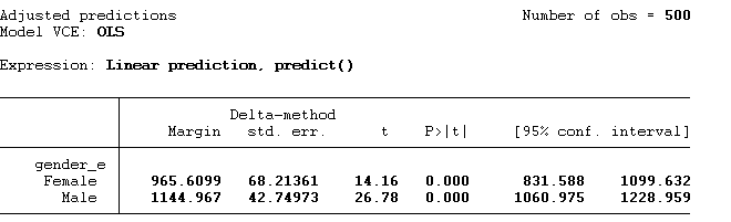
margin gender_e
This margin command will provide us with the predicted values of the dependent variable for the specific categories. The result of the above command is given below. Note: The values derived from the margin plots are consistent with the ones we obtained for the salary using the regression analysis, considering both the beta coefficients and the constant.
Once we get the margin values, we can plot them using the below command:
margins plot
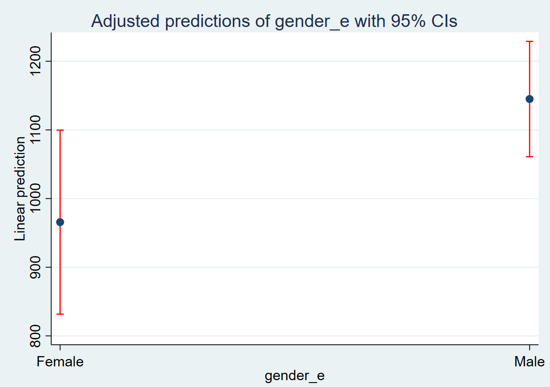
The graph is given below:
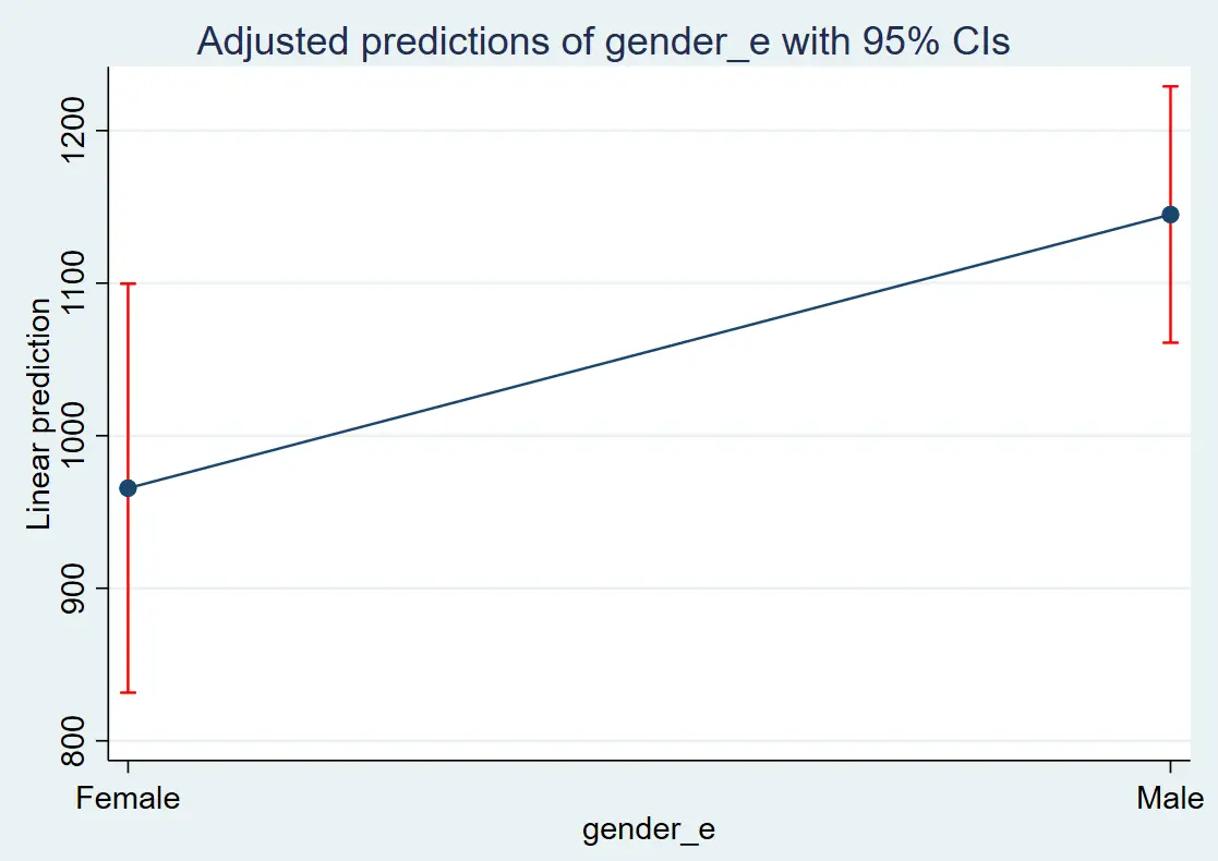
The red line is the confidence interval. From this graph, we can conclude that a male’s salary is higher than a female’s. To remove the blue line, we can use the below command:
marginsplot, recast(scatter)
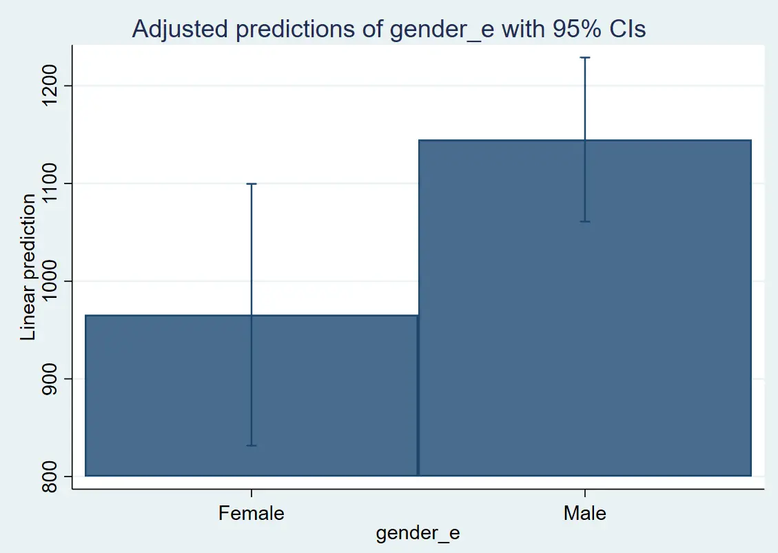
You will see that the blue line is removed. We can also show the predicted salary values for two categories using a bar chart. The command for the bar chart is given below:
marginsplot, recast(bar)