In our two-part article (Part1 , Part2) on the outreg2 command, we learnt how regression results from Stata can be output to other file formats like Word, Excel, and LaTeX. In this article, we delve into reporting results for panel regression models, specifically four regression models: OLS (fixed and random effects, Generalized Method of Moments and the Logit/Logisitc model.
For this guide, we will use the National Survey Data which is available online. To load this dataset we use
use http://www.stata-press.com/data/r16/nlswork.dta, clear
The option of clear indicates that any existing data in Stata’s memory will be cleared. It is always a good idea to describe the data and examine its format and other details through:
describe
OLS: Fixed Effects & Random Effects
Because fixed effects and random effect models are applied on panel datasets, we need to first declare our data as panel data.
xtset idcode year
This lets Stata know that it should treat our data as a panel dataset. The first variable after the xtset command is the cross-sectional/panel variable, while the second variable indicates what the time series variable is. Adding the time-series variable lets Stata order the panel observations by the time variable. So, in this example, the variable ‘idcode’ will be ordered based on the sequence of the variable ‘year’.
To run a simple OLS regression and output its results, we use:
regress ln_wage tenure ttl_exp grade outreg2 using results, word replace dec(3) ctitle(OLS)
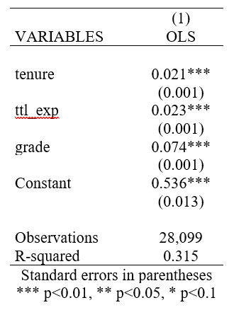
The dec(3) option specifies that all statistics should be displayed up to three decimal places. ctitle(OLS) ensures that the column title should be ‘OLS’.
Now, let’s run random effects and fixed effects regression models and output their results.
xtreg ln_wage tenure ttl_exp grade,re outreg2 using results, append dec(3) ctitle(Random Effect) xtreg ln_wage tenure ttl_exp grade,fe outreg2 using results, word append dec(3) ctitle(Fixed Effect) addtext(Country FE, YES, Year FE, YES) title(Results for OLS, Fixed and Random Effect) label noni
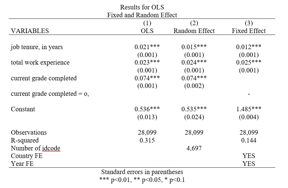
Note that we use the same filename ‘results’ to output all three results. The append option in the subsequent two regression ensures that their results are added to the file (instead of replacing it). The label ensures that the output table displays variable labels instead of names as variable labels are often easier to understand.
The addtext() option here adds text at the end of the regression table in a new row(s). For this option, we first write the legend name (the row title in the table) and after a comma, follow it by the text that we want in front of it. In this example, we use it to indicate the presence of ‘Country’ and ‘Year’ fixed effects.
This is different from the addnote() option which adds text at the bottom of the table as a note.
By default, Stata also outputs the number of groups in the cross-sectional/panel variable. If we wish to omit that from our table, we specify the option noni.
Generalized Method of Moments
Though several commands exist to help us run a GMM model, we employ the user written command xtabond2. Then we are going to report the regression results in ms word.
xtabond2 ln_wage l.ln_wage tenure ttl_exp grade, gmm(L1.(ln_wage)) iv(tenure ttl_exp grade) robust
A GMM regression output reports some extra statistics, such as the AR(1) and AR(2) values, and the Hansen and Sargan statistics. Sometimes we also require the number of instruments to be reported. In order to add all these statistics to our output table, we make use of the addstat() option:
outreg2 using results, replace word dec(3) addstat(AR(1),e(ar1p), AR(2), e(ar2p), Hansen, e(hansenp), Sargan, e(sarganp), Number of Instruments, e(j))
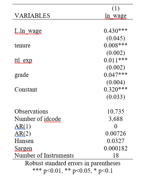
We report the AR(1), AR(2), the Sargan and the Hansen statistics through the addstat() option. The option requires us to first write the name of the variable the way we want it to appear in the table, followed by a comma, which is then followed by the macro name of the respective variable whose statistic we need reporting. We add as many variable names and their respective macros as we want, all separated by a comma.
Macros are temporary variables in Stata that store regression and summary statistics. They can be used to access specific statistics right after we run a regression. To access these variable names, we use either of the following commands:
ereturn list
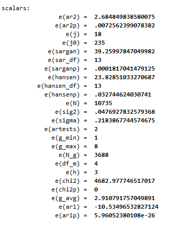
This returns a list of all the macros storing different regression related statistics along with their values.
Or we can use
help xtabond2
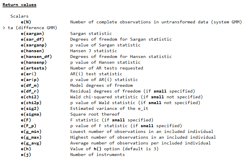
This opens the documentation for the xtanbond2 command. Under the heading of ‘Return Values’, it provides a list of the macros available after the regression and what statistics each macro stores. For example, e(sargan) stores the Sargan statistic.
Finally, we would like the table to limit the number of decimal places for all these statistics to three. To incorporate this, we use the adec() option, with the number of required decimal places in the parenthesis.
outreg2 using results, replace word dec(3) addstat(AR(1),e(ar1p), AR(2), e(ar2p), Hansen, e(hansenp), Sargen, e(sarganp), Number of Instruments, e(j)) adec(3)
Logit/Logistic Model
In a logit/logistic model, the dependent variable is categorical and binary (coded 0 and 1). The logistic model returns the odds ratios while the logit model returns the regression coefficients (log of odd ratios).
For this example, we will load a new dataset where we have a binary variable as the dependent variable. We will also describe the data.
webuse lbw describe
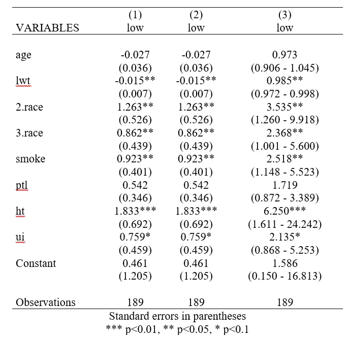
We note that, among other variables, ‘low’ is a byte variable. It takes a value of 1 if the birth weight is less than 2500g, and 0 otherwise. Summarizing the data using summ also shows maximum value of 1 and a minimum value of 0, indicating that it is indeed a binary variable. We use ‘low’ as a dependent variable and run and output the following logit regression.
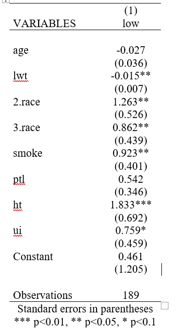
logit low age lwt i.race smoke ptl ht ui outreg2 using results, replace word dec(3)
We now use the logistic command to carry out our regression:
logistic low age lwt i.race smoke ptl ht ui outreg2 using results, append word dec(3)
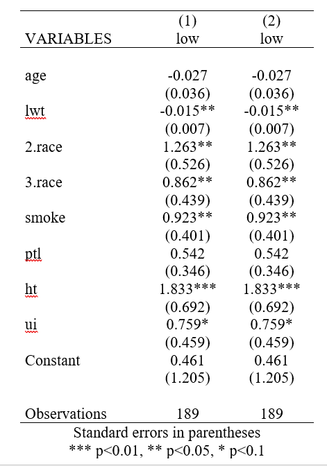
Having appended the results from this to the results from the first logit regression, we note that there is no difference in the statistics reported in the two columns. This is because we need to add the option eform for it to output the odds ratios (instead of log of odds ratios).
We also add two other options: ci to report confidence intervals; nodepvar to omit the inclusion of the dependent variable.
outreg2 using results, append word dec(3) eform nodepvar ci