
MANOVA stands for Multivariate ANalysis Of VAriance is an extension of ANOVA. In ANOVA we have only one dependent variable but in MANOVA we have more than one dependent variable to include. It is used to test the differences between multiple factors of independent variables. MANOVA allows us to check the difference between different factors of dependent variables caused by independent variables.
Assumptions of MANOVA
ANOVA and MANOVA have some assumptions that are the same except that they have to be extended for multivariate cases. You can check for assumptions in our previous article for ANOVA. The first assumption which is considered to be met is normality. Data must be normally distributed within each group of dependent variables. One can use the mshapiro.test() from mvnormtest package to test multivariate normality. The next assumption is homogeneity which means that variance across all the groups must be homogenous. Linearity also has to be taken into account in the case of performing MANOVA. It means that the independent variable must be linearly correlated with the various groups of dependent variables.
Example
Suppose we want to check the effect of different teaching modules on student’s performance. We took three different methods for this i.e. “Lectures, Workshops, and Online Study”. These methods will be tested on three different subjects “English, Math, and Physics”. This score variable will be our dependent variable with three subject’s scores. We will apply MANOVA to check how teaching methods impact student’s academic performance across multiple subjects.
Hypothesis
Hypothesis is to be tested to determine whether there is a significant difference in the scores of three subjects among different teaching methods. Below is the code for MANOVA.
Ho: µ1=µ2=µ3
H1: At least one teaching method is different.
Here µ is for different teaching modules.
# Load necessary libraries library(MASS) set.seed(123) n <- 500 # Number of students # Generate teaching method data TeachingMethod <- sample(c('Lectures', 'Workshop', 'Online'), n, replace = TRUE) # Generate marks for English, Math, Physics. marks_english <- sample(20:100, n, replace = TRUE) marks_math <- sample(20:100, n, replace = TRUE) marks_physics <- sample(20:100, n, replace = TRUE) # Create a data frame data <- data.frame( id = 101:(100 + n), TeachingMethod = TeachingMethod, marks_english = marks_english, marks_math = marks_math, marks_physics=marks_physics) # Display the first few rows of the resulting data frame head(data) # MANOVA analysis manova_result <- manova(cbind(marks_english, marks_math, marks_physics) ~ TeachingMethod, data = data) # Print the results summary(manova_result) 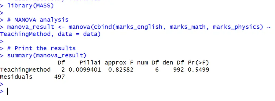
Pillai’s value ranges from 0 to 1. If the value of Pillai is near one shows a stronger relationship between dependent variables and independent variables. In the above case its value is too low which shows that teaching methods do not much explain the variation in combined independent variable. We are checking the null hypothesis that there is no significant difference in scores of different subjects among different teaching modules. Here p-value is greater than the significant level 0.05. It suggests that we do not have enough evidence to reject the null hypothesis. Results are insignificant in this case. So we conclude that there is no significant difference in combined scores of three subjects in between three different teaching methods. Insignificant results here do not meant that there is no difference in different teaching methods instead it means that we do not have enough evidence to assert that there is difference based on given sample.