
ANOVA, or ANalysis Of VAriance, is a statistical practice for confronting means over groups. It is an abstraction of t-test which is used for comparing the means of two groups. When we are coping with groups more than two we move ahead to ANOVA. It assesses whether there are any statistically significant differences in the means of three or more irrelevant (independent) groups.
It examines the variances of various groups. ANOVA splits the overall variance observed in a dataset into two segments: “Variance between groups and Variance within groups”. If the variance between groups is much enhanced than the variance within groups, it implies that the means of the groups deviate.
Basic Assumptions for ANOVA
ANOVA, like each statistical test, has precise assumptions that must be run for the results to be rational. The following are the essential assumptions of ANOVA:
- Observation Independence:
Each group’s observations are predicted to be independent of one another. In other words, data points from one group should not be associated to or dependent on data values from another group. Consider a study that analyzes the impact of three varied teaching strategies (A, B, and C) on student conduct in a statistics course. The treatment group is a three-level categorical variable (A, B, and C). Each level demonstrates a separate type of command. The hypothesis could be that the three teaching approaches have a substantial difference in mean student performance. We can see that every observation of these three methods does not affect one another. They are independent.
- Normality:
Among each category, the data should be almost normally distributed. ANOVA, on the other hand, is resilient to violations of normality, especially with higher sample sizes. Let’s consider this generated height data of men, women, and children for understanding the assumption of normality.
# Set seed for reproducibility set.seed(123) # Generate example data for three groups heights_group1 <- rnorm(30, mean = 170, sd = 5) heights_group2 <- rnorm(30, mean = 175, sd = 5) heights_group3 <- rnorm(30, mean = 180, sd = 5) # Combine data into a data frame height_data <- data.frame( height = c(heights_group1, heights_group2, heights_group3), group = rep(c("Men", "Women", "Children"), each = 30)) # Perform one-way ANOVA height_anova <- aov(height ~ group, data = height_data) # Check normality of residuals residuals_height_anova <- residuals(height_anova) shapiro_test_height <- shapiro.test(residuals_height_anova) # Print the result of the Shapiro-Wilk normality test cat("Shapiro-Wilk Normality Test for Heights:\n") cat("Test Statistic:", shapiro_test_height$statistic, "\n") cat("P-value:", shapiro_test_height$p.value, "\n")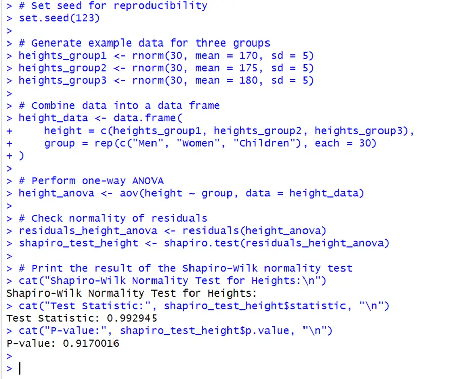
The Shapiro-Wilk test has a p-value 0.917, which is higher than the significant level 0.05. This implies that there is insufficient indication to reject the null hypothesis of normality. The residuals emerge to have a normal distribution.
- Variance Homogeneity (Homoscedasticity):
The variances of the several groups should be more or less equal. This is indicated to as variance homogeneity. In ANOVA, breach of this assumption can have an influence on the accuracy of the F-test. One can use the below code to check homoscedasticity.
plot(fitted(height_anova), residuals_height_anova, main = "Residuals vs Fitted", xlab = "Fitted values", ylab = "Residuals", col = "blue", pch = 16)
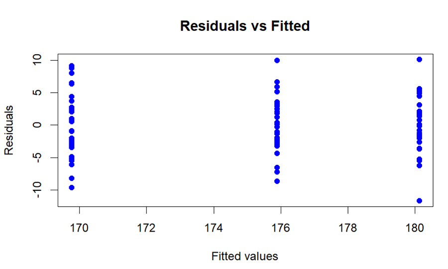
It can be seen in the plot that the variances are almost equal so we can consider this assumption fulfilled.
We can also use the Breusch-Pagan test for homoscedasticity. See the code below:
library(lmtest) bptest(height_anova)
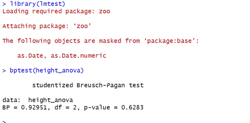
Null hypothesis of equal variances cannot be rejected as p-value is greater than specified significance level 0.05. So we conclude that there is homoscedasticity in data.
If the assumption of equal variances for one-way ANOVA is not met one can use welch ANOVA, which is an alternative to one-way ANOVA.
There are different types of ANOVA but we will discuss one-way ANOVA and two-way ANOVA in this article.
- One-way ANOVA:
One-way ANOVA is a statistical practice used to define whether there are any statistically significant differences in the means of three or more independent (unrelated) groups. It examines the variability within each group against the variability between groups to see if there is satisfactory evidence to reject the null hypothesis, which claims that there is no significant differences between group means.
Ho: µ1= µ2= ,…,=µn
H1: At least one mean is different.
Consider the above example to understand this concept.
# example data set.seed(123) # Generate example data for three groups heights_group1 <- rnorm(30, mean = 170, sd = 5) heights_group2 <- rnorm(30, mean = 175, sd = 5) heights_group3 <- rnorm(30, mean = 180, sd = 5) # Combine data into a data frame height_data <- data.frame( height = c(heights_group1, heights_group2, heights_group3), group = rep(c("Men", "Women", "Children"), each = 30)) # Perform one-way ANOVA height_anova <- aov(height ~ group, data = height_data) # Summarize the ANOVA results summary(height_anova)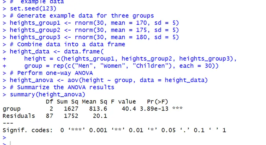
We can see from the output that groups of heights has an incredibly small p-value (3.89e-13), expressing that there is a considerable difference between at least one pair of groups (male, female/ male, children/ female, children).
In conclusion, the group variable has a considerable effect on the dependent variable height, and one may want to execute post-hoc tests to see whether individual groups differ from one another.
Regression
A one-way ANOVA is used to compare the means of distinct groups. However the one-way ANOVA can be designed as a simple linear regression model with a categorical predictor regarding regression.
Here’s an example of how to use the ‘lm()’ function in R to get the regression coefficients for a one-way ANOVA:
# Create example data set.seed(123) # Generate example data for three groups heights_group2 <- rnorm(30, mean = 175, sd = 5) heights_group3 <- rnorm(30, mean = 180, sd = 5) # Combine data into a data frame height_data <- data.frame( height = c(heights_group1, heights_group2, heights_group3), group = rep(c("Men", "Women", "Children"), each = 30)) # Perform linear regression regression_model <- lm(height ~ group, data = height_data) # Display regression summary summary(regression_model)The regression model output (‘lm’) embraces information about the estimated coefficients, standard errors, t-values, and p-values. Let’s release the output’s essential component:
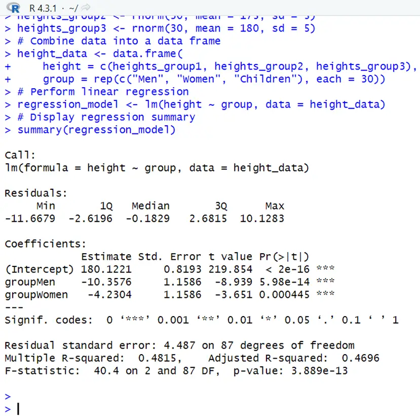
The anticipated change in height for people in the “Men” group (relative to the children group) is -10.3576 units. Statistically significant p-value, indicating that there is a noteworthy height difference between men and the control group children. A low p-value indicates that at least one predictor variable influences the response variable significantly. The regression model tells that the group variable has a considerable influence on the responding variable height.
Two-way ANOVA:
Two-way ANOVA, usually identified as two-factor ANOVA, is a statistical approach for examining the consequences of two independent factors on a dependent variable. It allows researchers to explore the interaction of two variables and evaluate whether or not they have a considerable impact on the outcome variable. Hypothesis for two way ANOVA are
- Ho: There is no statistically significant difference between means of Factor A.
Ho: μA1=μA2=⋯=μAi
H1: Factor A has at least one different mean.
- Ho: There is no statistically significant difference between means of Factor B.
Ho: μB1=μB2=⋯=μBi
H1: Factor B has at least one different mean.
- Ho: There is no interaction between Factor A and Factor B.
Ho: μA1B1=μA2B2=⋯=μAiBi
H1: Factor A and Factor B have an interaction effect.
In order to perform a two-way ANOVA in R, the model must be broadened to include two independent variables. You must use your own dataset for results.
# Set seed for reproducibility set.seed(123) # Generate example data for two factors exam_scores_math <- rnorm(30, mean = 70, sd = 10) exam_scores_english <- rnorm(30, mean = 75, sd = 10) exam_scores_physics <- rnorm(30, mean = 80, sd = 10) # Define factor levels student_grades <- rep(c("A", "B", "C"), each = 30) study_hours <- rep(c("Low", "High"), each = 45) # Combine data into a data frame exam_data <- data.frame( exam_score=c(exam_scores_math, exam_scores_english, exam_scores_physics), grade = factor(student_grades), study_hours = factor(study_hours)) # Perform two-way ANOVA exam_anova <- aov(exam_score ~ grade * study_hours, data = exam_data) # Summarize the ANOVA results anova_summary <- summary(exam_anova) # Print the ANOVA summary cat("Two-Way ANOVA Summary for Exam Scores:\n") print(anova_summary)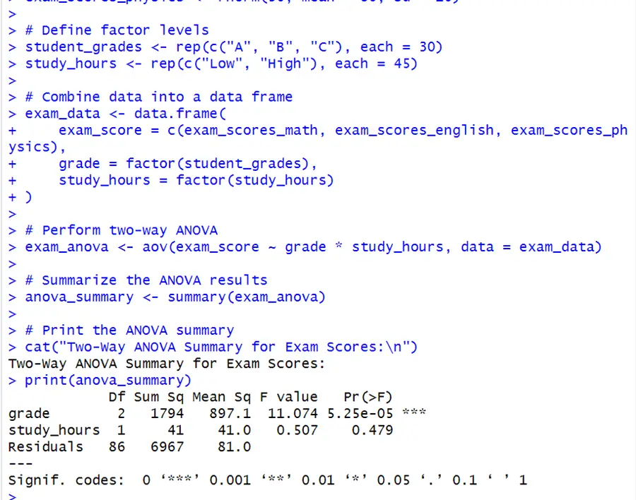
The Grade variable has a considerable effect on exam scores, conversely the Study Hours does not. This result does not clearly manifest the interaction effect between grades and study hours but it is vital to note. We may look at the validity of the interaction term (grade*study hour) in the model by plotting it. We will use the code below.
interaction.plot(exam_data$grade,exam_data$study_hours, exam_data$exam_score)
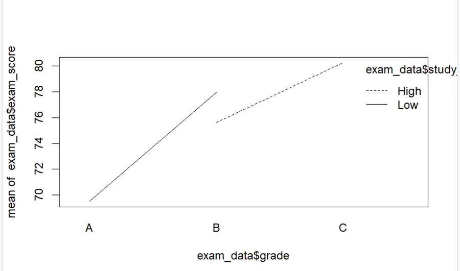
It can be seen that these lines have no interaction between them representing insignificance of results.
Regression in terms of Two-Way ANOVA:
The coefficients of a multiple linear regression model signifies the estimated influence of each independent variable on the dependent variable while governing for other variables in the model. A two-way ANOVA model can be idea of a type of regression in which categorical variables are incorporated as factors.
To fit a linear model in R, we can use the ‘lm()’ function to obtain the regression coefficients directly. Here’s an example of random dataset.
# Set seed for reproducibility
set.seed(123) # Generate example data for two factors exam_scores_math <- rnorm(30, mean = 70, sd = 10) exam_scores_english <- rnorm(30, mean = 75, sd = 10) exam_scores_physics <- rnorm(30, mean = 80, sd = 10) # Define factor levels student_grades <- rep(c("A", "B", "C"), each = 30) study_hours <- rep(c("Low", "High"), each = 45) # Combine data into a data frame exam_data <- data.frame( exam_score = c(exam_scores_math, exam_scores_english, exam_scores_physics), grade = factor(student_grades), study_hours = factor(study_hours)) # Perform regression regression_model <- lm(exam_score ~student_grades*study_hours , data =exam_data) # Display regression summary summary(regression_model)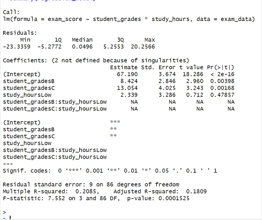
When comparing grade B students to grade A students, the expected change in exam score is 8.424 units. This coefficient is statistically significant as (p-value = 0.00398) is less than 0.05 , indicating that there is a substantial difference in exam scores between students who received a B grade and those who received an A grade. The F-statistic here evaluates the model’s overall significance. The p-value (0.0001525) in this case is less than 0.05, indicating that at least one of the predictors has a significant effect on the exam scores. According to the model above, student grades have a substantial influence on exam scores, but the effect of study hours is insignificant. The interaction terms have missing values (NAs), which may signal multicollinearity difficulties. The difference between ANOVA and regression is that anova contains interaction terms but regression model does not.
One should remember to take the p-values linked with each coefficient into account when determining their significance. A low p-value (usually less than 0.05) for a coefficient indicates that the variable is statistically significant in predicting the dependent variable.
If ANOVA reveals significant differences in group means, post-hoc tests (such as Tukey’s test) can be used to resolve which individual groups diverge from one another. ANOVA does not specify which groups are different; it simply indicates that there is a significant difference someplace.