
Time series analysis is a method of examining a set of data points collected over a period of time. Time series analysis implies analysts recording data points at constant intervals over an established span rather than just periodically or arbitrarily. It is simple to attain using the ts() method and certain parameters. Time series use a data vector and integrate each data point with a period value specified by the user. This function is usually used to discover and forecast the actions of a business asset over time.
Stock market prices are a real-world example of time-series data. The value of stocks, commodities, and other financial instruments is documented over time in financial markets. Each data point shows the asset’s price at a certain point in time. Analyzing historical stock prices as a time series can assist investors and analysts in identifying trends and patterns, as well as forecasting future price movements.
It is widely used in a variety of industries, including weather forecasting, energy usage prediction, flow of traffic analysis, and a lot more, where data is accumulated over time to grasp patterns and make educated choices.
To perform time series analysis in R, one can take help from the below example. Data has been created by the seq() function.
# Load necessary packages install.packages(c("forecast", "tseries")) library(forecast) library(tseries) # Set seed for reproducibility set.seed(123) # Create a time sequence from January 2020 to December 2022 with monthly frequency date_sequence <- seq(as.Date("2020-01-01"), as.Date("2022-12-31"), by = "months") # Create a linear trend with some random noise linear_trend <- seq(50, 150, length.out = length(date_sequence)) random_noise <- rnorm(length(date_sequence), mean = 0, sd = 10) stock_prices <- ts(linear_trend + random_noise, start = c(2020, 1), frequency = 12) stock_prices # Plot the generated time series plot(stock_prices, main = "Stock Prices Data", xlab = "Date", ylab = "Values")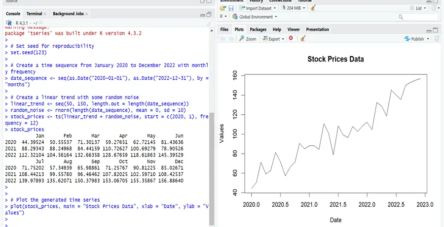
It can be seen in the picture that values have been generated against 3 years as monthly data and a time series graph that shows stock prices vs. years.
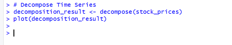
Now we will decompose the dataset into its components, i.e., trend, seasonal, and noise. You can use the code below for decomposition.
# Decompose Time Series decomposition_result <- decompose(stock_prices) plot(decomposition_result)
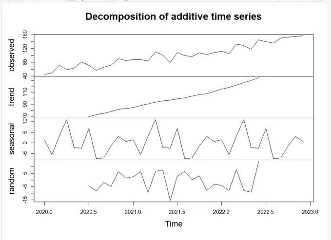
In the above graph, there are four parts. The first part shows all the data patterns in the observed graph, and the remaining three graphs contain the values with trend, seasonality, and random noise.
ACF and PACF
ACF (Autocorrelation Function) and PACF (Partial Autocorrelation Function) are time series analytic methods used to understand and quantify autocorrelation in data. They are used to figure out the order of AR, MA and ARMA for forecasting points of view.
1. ACF (Autocorrelation Function):
ACF gauges the relationship between a time series and its lag values. It fosters identifying patterns in data, such as seasonality or trends. The ACF at lag (k) is the correlation between the values of the time series at time (t) and the values at time (t-k). The ACF function can be employed to determine the order of a moving average (MA) process. Normally, the ACF is shown as a function of lag, depicting how the correlation between observations drops as the dromancy grows.
2. PAF (Partial Autocorrelation Function):
PACF calculates the correlation between a time series and its lagged values after accounting for intermediate lags. It aids in assessing the direct relationship between observations made at different times. The PACF at lag (k) is the correlation between the time series values at time (t) and values at time (t-k), corrected for the influence of lags (1-k). The PACF function can be used to determine the order of an autoregressive (AR) process.
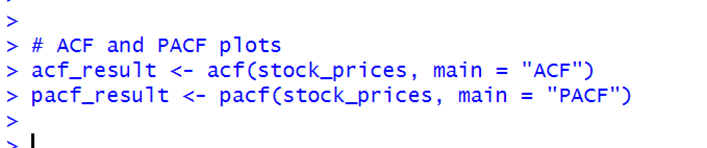
# ACF and PACF plots acf_result <- acf(time_series_example, main = "ACF") pacf_result <- pacf(time_series_example, main = "PACF")
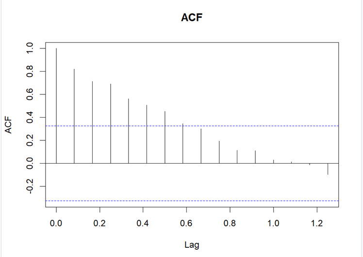
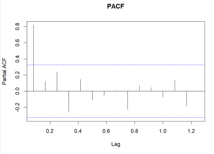
In above plots, there are abundant spikes at different lags (k) which show a correlation between observations at time (t) and (t-k). There is no need to look at the spike at lag 0.
The overall behavior of this ACF plot is exponential. ACF with exponential decay suggests an AR process. Whereas ACF with a cutoff after lag q suggests an MA process. PACF has two significant spikes, which shows that the process is AR(2).
Modeling and forecasting with ARIMA
The auto.arima function from the forecast package is used to set the appropriate ARIMA model with the best parameterization. Below is the code for this function.
# Fit ARIMA model arima_model<- auto.arima(time_series_example) print(arima_model) # Forecast using ARIMA model # Forecasting for the next 12 months forecast_values <- forecast(arima_model, h = 12) plot(forecast_values, main = "ARIMA Forecast", xlab = "Date", ylab = "Values") # Evaluate forecast accuracy accuracy(forecast_values)
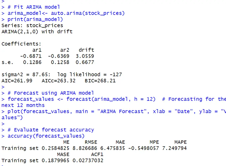
The ARIMA model captures a linear trend (1st differencing) with two autoregressive terms (lag 1 and lag 2) and a drift term. The forecast reliability measurements indicate reasonable accuracy.
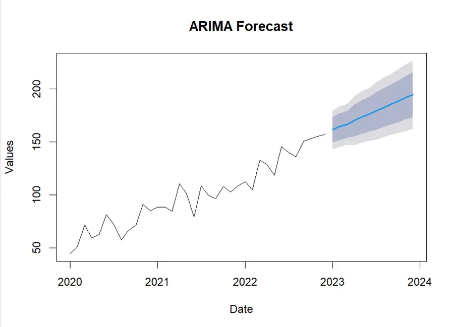
The highlighted part of the above graph, which is increasing, shows the forecast for stock prices for the next year.
Assumptions check
After modeling, testing assumptions assures that the chosen model is an adequate fit for the data. If, after modeling, the assumptions are not met, we may need to reconsider our model choices or explore additional modifications.
Below is the code to check some of the assumptions for this model.
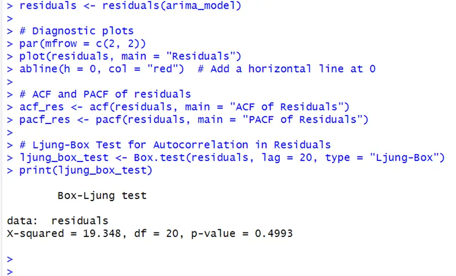
# Residuals from ARIMA model residuals <- residuals(arima_model) # Diagnostic plots par(mfrow = c(2, 2)) plot(residuals, main = "Residuals") abline(h = 0, col = "red") # Add a horizontal line at 0 # ACF and PACF of residuals acf_res <- acf(residuals, main = "ACF of Residuals") pacf_res <- pacf(residuals, main = "PACF of Residuals") # Ljung-Box Test for Autocorrelation in Residuals ljung_box_test <- Box.test(residuals, lag = 20, type = "Ljung-Box") print(ljung_box_test)
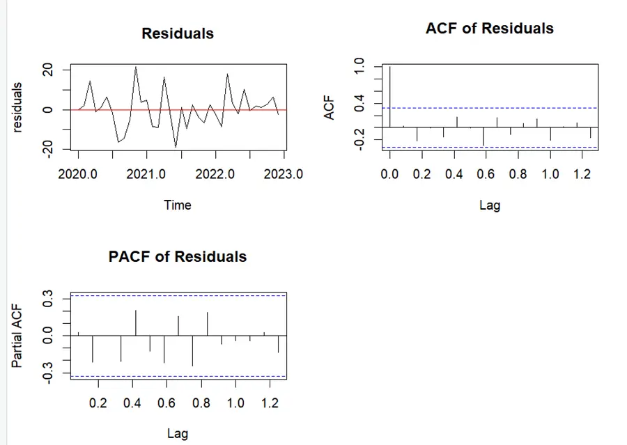
There is no apparent trend or seasonality shown in the residual vs. time graph. Ideally, the ACF of residuals does not show significant autocorrelations at any lag, indicating that there is no remaining systematic pattern in the residuals. Similarly, the PACF of residuals did not exhibit significant spikes, indicating that there is no remaining pattern after accounting for the earlier lags.
The next assumption is checked by the Ljung-Box test, which is a residual autocorrelation test. The null hypothesis for this example is that there is no autocorrelation in the residuals.
The p-value is 0.4993, which is greater than the standard level of significance of 0.05. As a result, the null hypothesis is not rejected.
This implies that there is no significant autocorrelation in the residuals, demonstrating that the ARIMA model effectively captured the time series’ temporal dependencies.
In summary, the findings show no evidence of considerable autocorrelation in the residuals, indicating that the ARIMA model is adequate for this time series.