
Stationarity is a primary principle in time series analysis. A time series is considered to be stationary if its statistical aspects, such as mean, variance, and autocorrelation, remain constant through time. To elucidate, the time series does not reflect trends, seasonality, or other regular patterns that alternate with time.
Stationarity is essential in time series analysis because it upholds many statistical techniques and models. For example, classical linear regression models infer a constant mean and variance, but autoregressive models infer a constant autocorrelation.
While working with a non-stationary time series, it is frequently essential to adapt it to a stationary series before the implementation of specific models or statistical tests. The usual means for establishing stationarity are:
1. Differencing: Subtracting the preceding observation from the present one can help eradicate tendencies.
2. Transformations: Using mathematical transformations such as logarithms or square roots to equalize variance.
3. Seasonal Adjustment: Removes seasonal tendencies from the data.
4. Detrending: Removes a trend component from a time series.
It’s noteworthy that in various cases, non-stationary behavior may be anticipated, and specialist models like integrated autoregressive moving average models (ARIMA) can handle this. Moreover, advances in time series analysis have resulted in the development of models capable of managing non-stationary data, such as long-term associations in cointegrated time series.
Visual examination, statistical testing, and the application of adequate transformations can all be used to discern stationarity and convert a non-stationary time series to a stationary one.
Certainly! Let’s employ R’s quantmod and tseries packages to work with stock exchange data. In this example, we’ll gather historical daily closing prices of a stock, check for stationarity using the Augmented Dickey-Fuller (ADF) test, and use differencing if necessary. Below is the code for this.
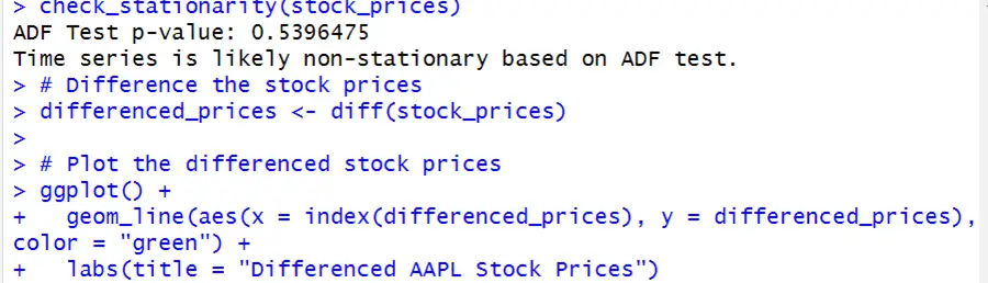
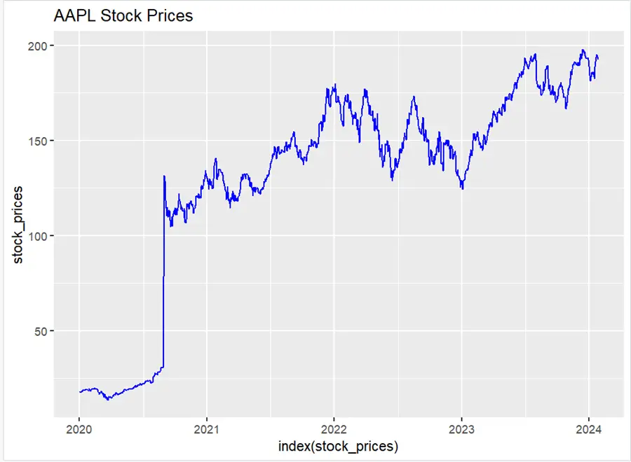
Install and load necessary packages install.packages(c("quantmod", "ggplot2", "tseries")) library(quantmod) library(ggplot2) library(tseries) # Function to check stationarity using ADF test check_stationarity <- function(ts_data) { adf_test_result <- adf.test(ts_data) cat("ADF Test p-value:", adf_test_result$p.value, "\n") if (adf_test_result$p.value < 0.05) { cat("Time series is likely stationary based on ADF test.\n") } else { cat("Time series is likely non-stationary based on ADF test.\n") } } # Download historical stock prices getSymbols("AAPL", from = "2020-01-01", to = Sys.Date(), src = "yahoo", adjust = TRUE) stock_prices <- Cl(AAPL) # Closing prices # Plot the stock prices ggplot() + geom_line(aes(x = index(stock_prices), y = stock_prices), color = "blue") + labs(title = "AAPL Stock Prices") # Check stationarity check_stationarity(stock_prices) If adf test imply non stationarity we can apply differencing # Difference the stock prices differenced_prices <- diff(stock_prices) # Plot the differenced stock prices ggplot() + geom_line(aes(x = index(differenced_prices), y = differenced_prices), color = "green") + labs(title = "Differenced AAPL Stock Prices") # Difference the stock prices differenced_prices <- diff(stock_prices) # Remove rows with missing values differenced_prices <- na.omit(differenced_prices) # Plot the differenced stock prices ggplot() + geom_line(aes(x = index(differenced_prices), y = differenced_prices), color = "green") + labs(title = "Differenced AAPL Stock Prices") # Check stationarity of differenced series check_stationarity(differenced_prices) The given R code runs time series analysis on historical stock prices for Apple Inc. (AAPL) received from the Yahoo Finance API. Primarily, key programs like as ‘quantmod’, ‘ggplot2’, and ‘tseries’ are installed and loaded to simplify data processing and visualization. The code delimits the function ‘check_stationarity’, which uses the Augmented Dickey-Fuller (ADF) test to ascertain the stationarity of a given time series. To accomplish a stationary time series, differencing is applied to the stock prices once stationarity is checked. The differenced series is then plotted to manifest the effect of differencing. Throughout the code, the ADF test results are presented to imply if the time series is likely to be stationary or not. Overall, the code sheds light on the stationarity of stock prices and demonstrates the transformation procedures required to produce a stationary time series for future research.
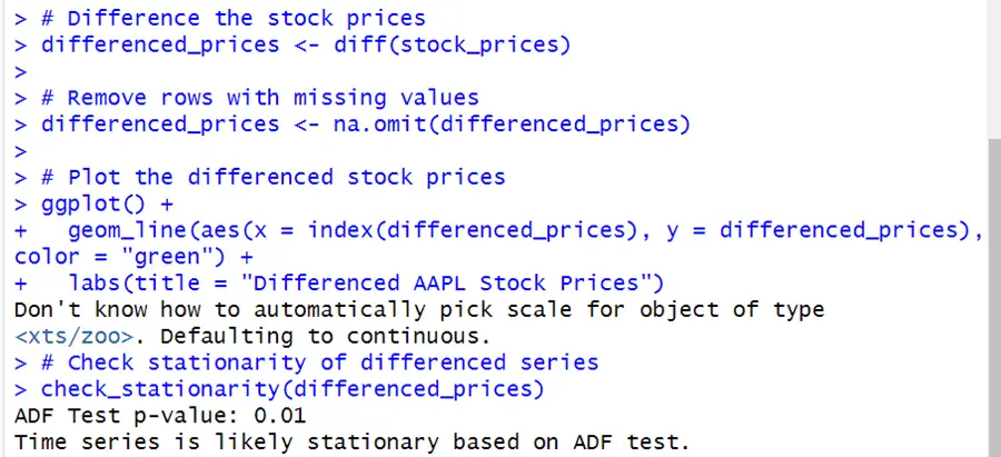
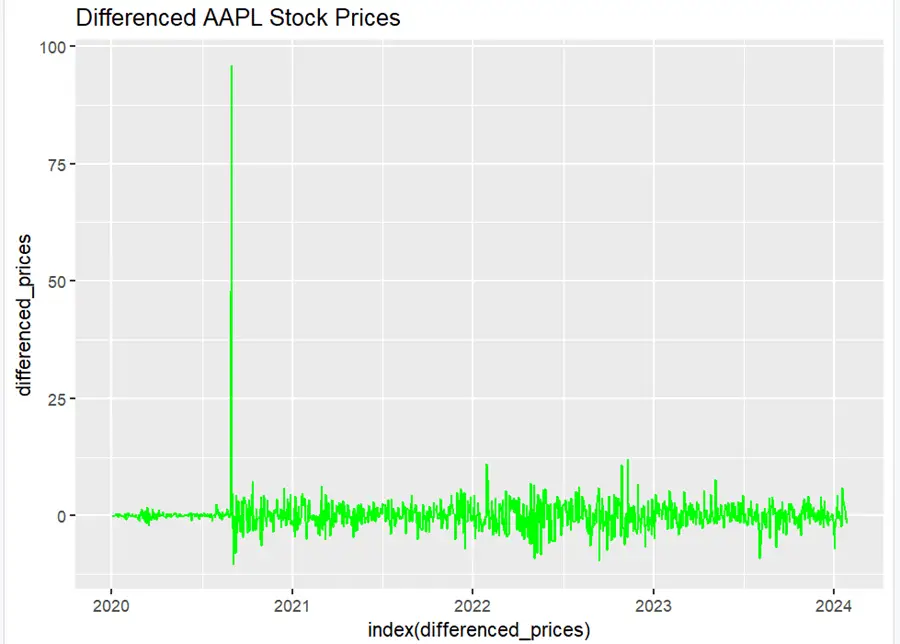
It can be seen in the graph that stationarity has been achieved.
The code for another method, like transformation, that can be used to make data stationary has been shown below.
# Load necessary packages install.packages(c("quantmod", "ggplot2", "tseries")) library(quantmod) library(ggplot2) library(tseries) # Function to check stationarity using ADF test check_stationarity <- function(ts_data) { adf_test_result <- adf.test(ts_data) cat("ADF Test p-value:", adf_test_result$p.value, "\n") if (adf_test_result$p.value < 0.05) { cat("Time series is likely stationary based on ADF test.\n") } else { cat("Time series is likely non-stationary based on ADF test.\n") } } # Download historical stock prices getSymbols("AAPL", from = "2020-01-01", to = Sys.Date(), src = "yahoo", adjust = TRUE) stock_prices <- Cl(AAPL) # Closing prices # Plot the original stock prices ggplot() + geom_line(aes(x = index(stock_prices), y = stock_prices), color = "blue") + labs(title = "AAPL Stock Prices") # Check stationarity check_stationarity(stock_prices) # 2. Mathematical Transformations: Applying Logarithmic Transformation log_transformed_prices <- log(stock_prices) # Plot the logarithmically transformed stock prices ggplot() + geom_line(aes(x = index(log_transformed_prices), y = log_transformed_prices), color = "purple") + labs(title = "Log-transformed AAPL Stock Prices") # Check stationarity of the log-transformed series check_stationarity(log_transformed_prices)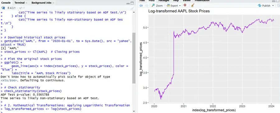
Stationarity has been acheived by log transformation. After a sudden rise in the stock prices in 2020 series became somehow stationary.