
What are Dummy Variables
Dummy variables, also called binary variables, are variables that only take two values: 0 and 1. Such variables are often used to quantify qualitative data like gender, sector of work. city/country etc. For example, a variable called ‘female’ might equal 1 for observations on females and 0 for observations on male respondents in a survey.
More on how to create dummy variables in Stata can be found in our dummy variable guide.
Dummy variables are widely used in regressions, sometimes as dependent variables, sometimes as independent variables, and sometimes as both. In each case, the type of regression run and interpretations made will vary.
In this article, we will cover some cases where the dependent variable is a binary variable. This concept is well explained in Chapter 10 of Microeconometrics Using Stata by A. Colin Cameron.
For the regressions in this article, we will use Stata’s own dataset called ‘heartsm.dta’. The dataset can be loaded using the command:
use https://www.stata-press.com/data/r17/heartsm.dta
summ
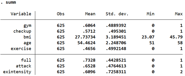
This is an individual-level dataset about people’s heart health and other health indicators. Variables ‘bmi’ and ‘age’ are continuous variables while ‘exintensity’ is a categorical variable with three categories. All other variables are binary/dummy variables.
Regressions with Dummy Dependent Variables and a Continuous Independent Variable
Linear Probability Model
Let’s run and interpret a regression where the dependent variable is a dummy variable which is regressed on a continuous independent variable. Such a model is also called the Linear Probability Model.
In this example, we are interested in seeing whether a person’s BMI is associated with heart attacks or not. Our dependent variable, ‘attack’ is a dummy variable which equals 1 if a person has had a heart attack and 0 otherwise.
reg attack bmi
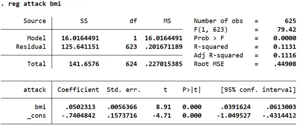
The coefficient on ‘bmi’ suggests that for a 1 unit increase in a person’s BMI, the probability of having a heart attack goes up by 0.05 or 5%. This is also statistically significant at the 5% level as the p-value is 0.00.
However, a simple OLS regression is not appropriate when the dependent variable takes on binary, 0/1 values. This is because, in such a setup, the interpretation of the coefficient (and predicted values) is in terms of probabilities. But because OLS is linear in the parameters it predicts, this implies that some predicted values might go over 1 which makes no sense when interpreting them as probabilities.
Related Article: Regression Assumptions in Stata for Beginners
Let’s obtain the predicted values and summarize them.
predict attack_hat summ attack_hat
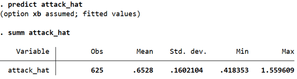
The maximum value taken by the fitted values for ‘attack; is 1.56. This is wrong and cannot be interpreted as a probability in a sensible manner. Additionally, the variance of the error term in this model will also be non-constant i.e the model will have heteroskedasticity. For all observations, the predicted values should be greater than or equal to 0 or less than or equal to 1 (0 ≤ fitted value ≤ 1).
To address such a problem, we need to turn to non-linear regressions. These regressions restrict the outcome variable’s predicted value between 0 and 1 allowing us to interpret them as probabilities.
Non-Linear Regressions
Probit Model and Marginal Effects
A probit model is one type of regression model that can be run when you have a binary outcome variable. A probit model assumes that the probability of the outcome variable equalling 1 is determined by the standard normal cumulative distribution function.
A probit function maps outcome values between 0 and 1 to a corresponding value on the standard normal distribution, which allows for the estimated coefficients to be interpreted as the probability of the outcome being equal to 1.
probit attack bmi
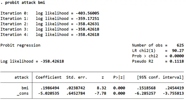
The coefficient outputs from a probit command represent the z-scores. They can give us an indication of the direction and size of the effect, but cannot be interpreted as probabilities directly. In this regression, the coefficient suggests that, on average, a one unit increase in a person’s BMI increases the chances of a heart attack. This effect is statistically significant as well as indicated by the p-value of 0.00.
This may be a positively biased estimate because we did not add other relevant variables like a person’s age or exercise regularity.
In order to obtain marginal effects that can be interpreted as probabilities, we use a post-estimation command called margin.
margin, dydyx(*)
The option dydx(*) tells Stata to estimate the marginal effect of all variables in the regression. If you had several covariates in your regression but only needed to report the marginal effects of a few, you could list those in place of the asterisk.
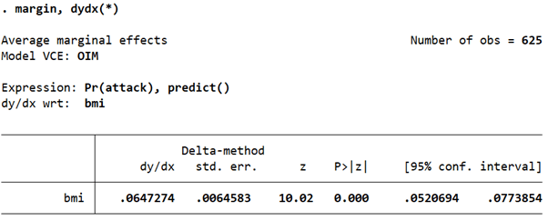
For each unit increase in a person’s BMI, the probability of a heart attack goes up by 0.065. Note that if we had added more covariates in our model, the marginal effect reported would have taken into account the control for them as well.
Later on in this article, we will see how using the margin command for categorical variable with more than two categories helps us understand the marginal effect of each unit increase in the variable on the outcome.
Logistic/Logit Model
Logistic/logit regression models are another popular choice for modelling binary dependent variables. A logistic regression outputs the odds ratios while a logit regression outputs the log of odds ratio or the log odds.
Output from the logit regression can also be turned into odds ratio by simply exponentiating the coefficient.
Which of these regressions you choose to run depends on whether you prefer to obtain odds ratios while others prefer the coefficients as log odds.
logit attack bmi
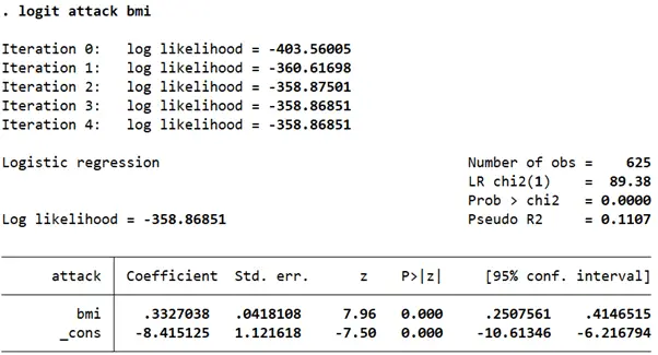
The results from this logit regression suggest that for a one unit increase in a person’s BMI, the log odds of a heart attack go up by 0.33. Since higher log odds correspond to higher probabilities, this again suggests that individuals with higher BMIs are more likely to have heart attacks.
Log odds is not always the most intuitive coefficient to interpret so it is more likely that researchers report the odds ratios (way more intuitive) when dealing with binary dependent variables.
To report the odds ratios, two commands can be used: the logit command with the option or, or the logistic command.
logistic attack bmi
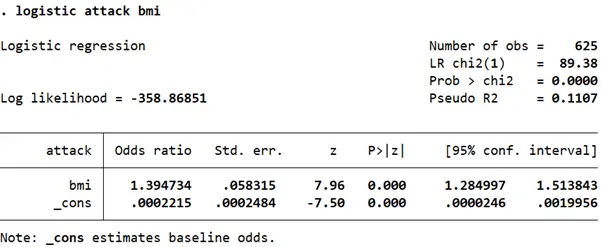
When we run the same regression using the logistic command, we interpret the output as the odds ratio of having a heart attack going up by 1.4 for each unit increase in BMI.
In other words, the odds of having a heart attack are predicted to increase by 1.4 times larger for each unit increase in one’s BMI.
If the difference between two people’s BMI is of 2 units, the person with the higher BMI has predicted odds of 1.4*1.4 (=1.96) of having a heart attack than the person with the lower BMI.
If their BMIs differ by 4 units, the odds that the person with the higher BMI will have a heart attack are calculated by 1.44 (=3.84). This means that their odds of having a heart attack are 3.84 times higher than the person with the lower BMI.
Related Article: How to Perform the ANOVA Test in Stata
Note: Odds ratios are never equal to 0. Odds ratios greater than 1 can be interpreted as “positive effects”. Odds ratios between 0 and 1 are interpreted as “negative effects”. When odds ratios equal 1, we conclude that the two variables have no association.
Regressions with Dummy Variables as Both Dependent and Independent Variables
It is also very common to have regression models where both your dependent and independent variables are binary. In such a case, the interpretation remains the same. The outcome variable is said to change whenever the independent variable equals 1. In the following example, we want to see the effect of exercising on the probability of a heart attack.
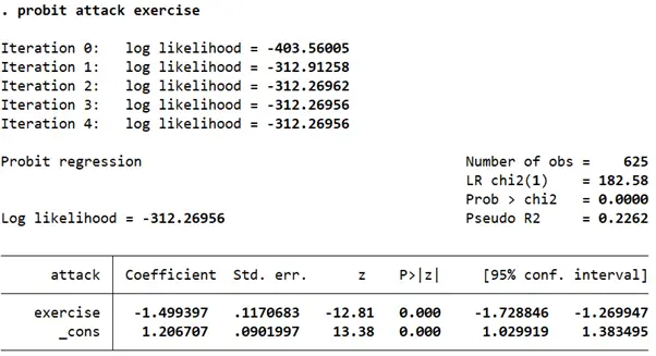
The negative and significant coefficient/z-score indicates that exercising reduces the probability of a heart attack.
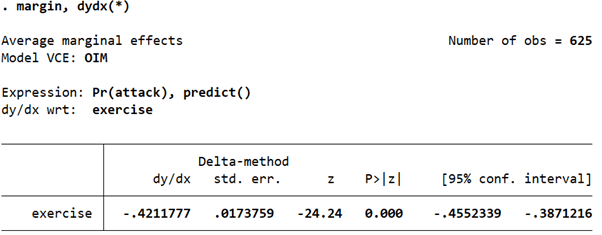
In terms of marginal effects, when exercise is equal to 1 i.e. for people who exercise, the probability of a heart attack goes down by 0.42 relative to those who don’t exercise.
We can also check the odds ratio for the same model.
logistic attack exercise
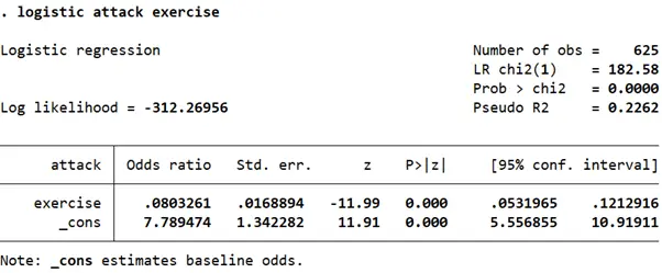
For people who exercise, the odds ratio of a heart attack is 0.08. Remember that an odds ratio of less than 1 indicates a negative effect. Or, in other words, the odds of a heart attack happening to the ‘exposed’ group (in this case, individuals for whom exercise equalled 1), are lower than those for whom exercise was equal to 0.
Regressions with a Categorical Variable as the Independent Variable
In regressions where your independent variable has more than two categories, the margin command comes in very handy to see how the effect on the outcome variable changes from one category to another. In our example, we will explore two such scenarios: one where the dependent variable is binary and one where it is continuous.
For the first one, let’s load a new dataset on high blood pressure data using the following command and summarize it.
use https://www.stata-press.com/data/r17/hbp.dta
summ
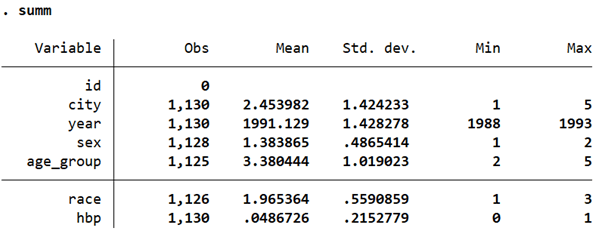
We can see that ‘hbp’, the variable for high blood pressure is a binary one. It takes on the value of 1 for people who have high blood pressure and 0 for those that don’t. All other variables, apart from ‘id’ and ‘year’ are categorical variables.
Before getting into regressions, we will rename the variable ‘sex’ to ‘male’ and change the coding of the variable such that females in the data take on the value of 0 instead of 2 like they do right now.
replace sex=0 if sex==2 rename sex male lab def sex 0"Female" 1"Male" lab val male sex codebook male
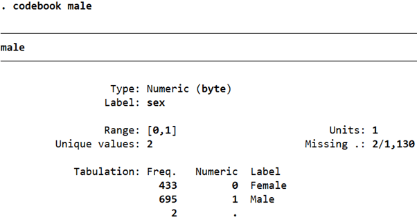
We have now turned this into a typical binary/dummy variable that takes on values of 0 and 1 only.
We would like to see the effect of a person’s gender and race on their probability of having high blood pressure. In this case, we will only use the probit command, but the process can be replicated using the logistic command as well.
probit hbp sex race margin, dydx(*)
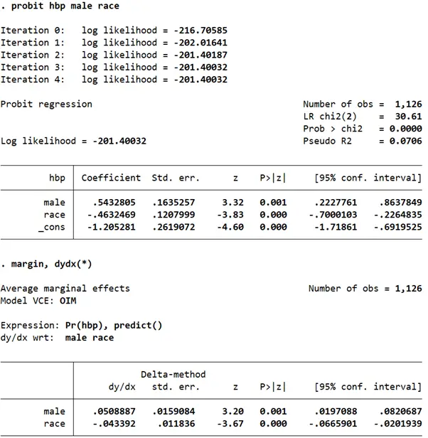
This suggests that males, controlling for race, have a 0.051 higher probability than females of having high blood pressure. The coefficient and marginal probability for race is a little difficult to interpret, however. The variable equals 1 for White, 2 for Black, and 3 for Hispanics.
To make a better interpretation of variables with more than one category, we can prefix them with ‘i.’. This prefix tells Stata that the variable is a categorical variable and we need it to report coefficients for each of the categories rather than one average effect like before.
Another optional alteration we will make to our command is the addition of the option allbaselevels. When this option is specified, Stata indicates which category is treated as the base category i.e. which category needs to be compared to when interpreting coefficients.
probit hbp male i.race, allbaselevels
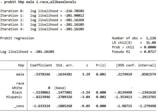
Now, our output table includes coefficients for two out of the three categories for race. Because Stata chose White as the base category, our interpretation of the other two coefficients for race will be made in comparison to White. Let’s report the marginal effects.
Related Article: Publication Style Regression Output in Stata
margin, dydx(*)
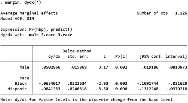
The marginal effect for males relative to females is still similar to our previous regression. As compared to females, males have 0.05 higher probability of having high blood pressure.
Black people, controlling for gender, have a 0.65 lower probability of having high blood pressure as compared to white people. Hispanic people have a 0.084 lower probability of having high blood pressure than white people while controlling for gender.
All three marginal effects are statistically significant.
Interaction Terms in Regressions
In examples similar to the above, it is often relevant to study how two variables interact and affect the outcome variable together. For example, it is very likely that gender and age interact together to affect the probability of high blood pressure.
We can ask Stata to display the interaction effects of two variables by writing one or two hash (#) signs between them. If we specify only one hashtag, Stata will output only the interaction effects. If we add two hashtags, Stata will report both the main effect for each variable and their interaction effect.
Let’s look at the main effects and the interaction effect of gender and the age group that a person belongs to. We use the allbaselevels option once again to report which categories (and pairs of categories) were dropped by Stata..
probit hbp male##age_group, allbaselevels
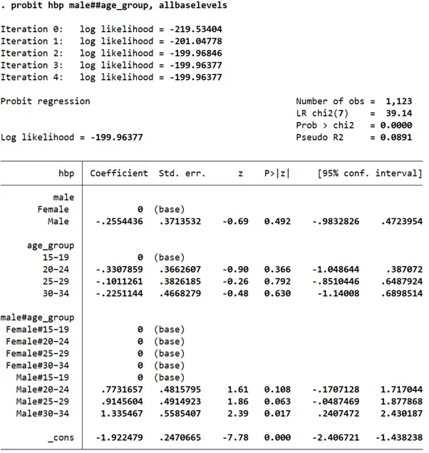
The main effect and interaction effects for the 15-19 age group and for females were dropped. The marginal effects are as follows:
margin male##age_group
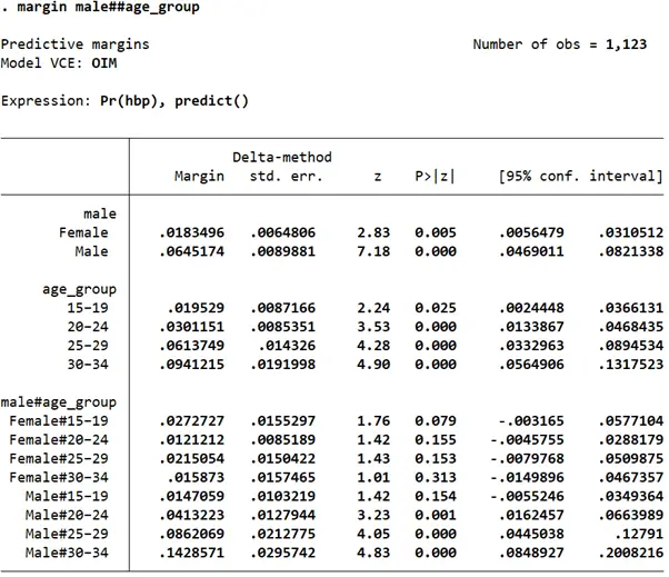
This table suggests that if everyone in the data would be treated as a male, their probability of having high blood pressure would be 0.065, while for females, this probability would be lower at 0.018.
If everyone in the data were treated as belonging to the 15-19 age group, their probability of having high blood pressure would be 0.0195 but as the age group increases, this probability also increases to 0.094 for the 30-34 age group.
Moving on to the interaction effects of the two-factor variables, the group with the lowest probability of having high blood pressure is that of females aged between 20-24 (probability=0.012). The group with the highest probability of having high blood pressure is males belonging to the 30-34 age group (probability=0.143).
Instrumental Variables and the Wald Estimator
In econometrics, the presence of an endogenous covariate (like treatment, for example) may lead researchers to resort to using instrumental variables (IVs). When an IV is a binary variable, the estimator is called the Wald Estimator.
Dummy variables are a very powerful tool in data analysis and causal inference research work. Knowing how to work with them is a useful tool to have in your skillset.