In our previous article, we delved into the fundamentals of creating dummy variables for binary categories, using gender—with its two categories of male and female—as a prime example. However, the landscape of categorical variables is far more expansive, often featuring more than two categories. In this follow-up article, we’ll broaden our focus to tackle categorical variables beyond binary, exploring how to seamlessly incorporate them into your regression models. We will explore the following topics:
- Single Categorical Regressor
- Multiple Categorical Regressors
- A Categorical and a Continuous Regressor
The same dataset will be used in this article.
Download Example File
Our last article focused on gender—specifically the categories male and female—as an example of incorporating binary categorical variables into regression models. This time, we’re shifting our lens to a more complex variable: education levels, which include ‘Bachelor,’ ‘Master,’ ‘Primary,’ and ‘Secondary.’ So, in this article, we will use education as our independent variable. Remember, before proceeding to the regression, we must encode the education variable to convert qualitative into quantitative categories. The command is given below:
encode education, generate(education_e)
After executing the command, the unique value will be assigned to each category. Now, we can proceed to the regression using the below command:
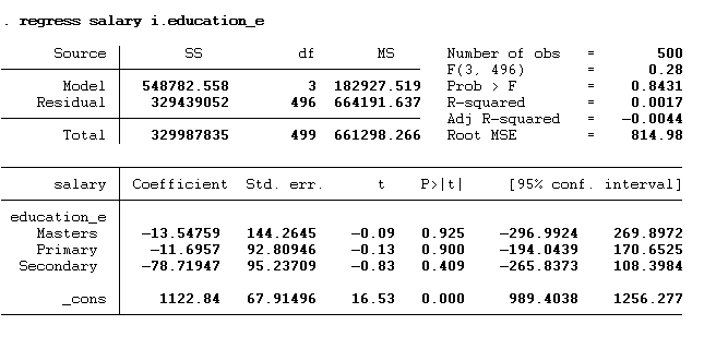
regress salary i.education_e
Remember to use the encoded variable education_e instead of the original string variable. The results are presented below:
Remember, we discussed the m-1 rule for the dummy variable in the previous article. According to that rule, one category is always omitted to prevent dummy trap error. To see which category has been omitted, we will use the allbaselevels option with the above command, as shown below:
regress salary i.education_e, allbaselevels
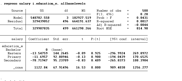
The results show that “bachelor’s” has been used as the base. The interpretation of all three other categories will always be with respect to the omitted category. Hence, the interpretation of the above results will be that individuals with a master’s degree would earn $ 13.55 less than individuals with a bachelor’s degree. Similarly, the primary degree holder would earn $11.70 less, and the secondary degree holder would earn $78.72 less than those holding a bachelor’s degree. The constant represents the predicted salary of the base category, which is a bachelor’s degree. These results do not depict real world situation as the data is hypothetical.
So, what happens if we are interested in comparing education levels directly against one another—say, ‘Master’ to ‘Primary,’ or ‘Secondary’ to ‘Primary,’ and so on? In that case, we will need to reconsider our base category, which is currently set as ‘Bachelor.’ Before making that shift, it’s important to understand how each category is numerically labeled. In Stata, categories are usually assigned labels in alphabetical order. In our example, ‘Bachelor’ is labeled as 1, followed by ‘Master’ with 2, ‘Primary’ with 3, and finally, ‘Secondary’ takes the label 4. But we need it differently. For example, we want to assign 1 value label to primary, 2 to secondary, 3 to bachelor’s, and 4 to master’s. To set the value labels use following command:
label define edu_label 1 "Primary" 2 "Secondary" 3 "Bachelor" 4 "Masters"
In the above command, we generate the label assigned to the new encoded variables. In this command, label define is the command, edu_label is the label’s name, and then we will write the code with value within the commas. After executing the above command, we will use the encode command again and assign these labels (edu_level) to that newly encoded variable. The command is given below:
encode education, generate(education_e) label(edu_label)
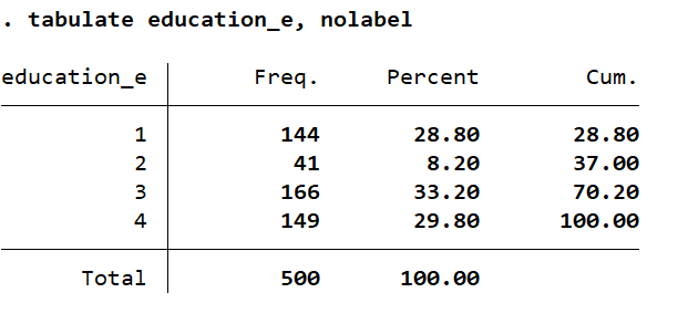
On executing the above command, the new encode variable will be generated using the label (1 = Primary 2 = Secondary 3 = Bachelor 4 = Masters) we had asked Stata to use.
tab education_e tab education_e, nolabel
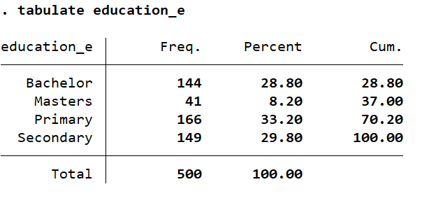
The label has been assigned, as we want it to be. We will execute the regression command again:
regress salary i.education_e, allbaselevels
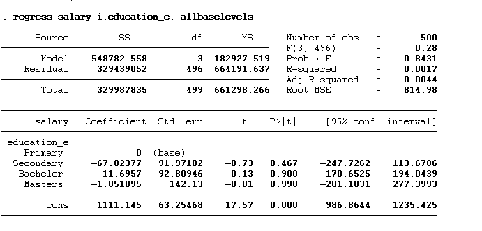
Now, the base or omitted category is “primary”. We will interpret these findings as an individual holding a secondary degree would earn $67.03 less than an individual holding a primary degree. The bachelor’s degree holder would earn $11.70 more, and the master’s degree holder would earn $1.85 less than the individual holding the primary degree.
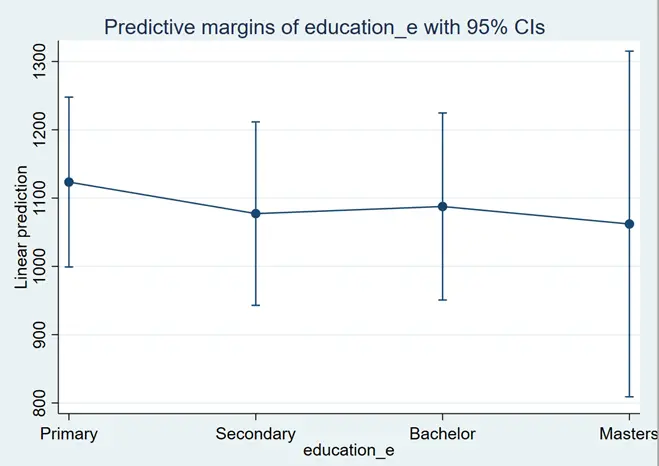
We can also visualize our results using the margin plot used in the previous article. The commands are given below:
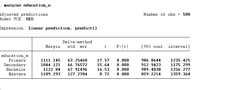
margins education_e
The above command will provide us with the predicted value, of each category, as shown below:
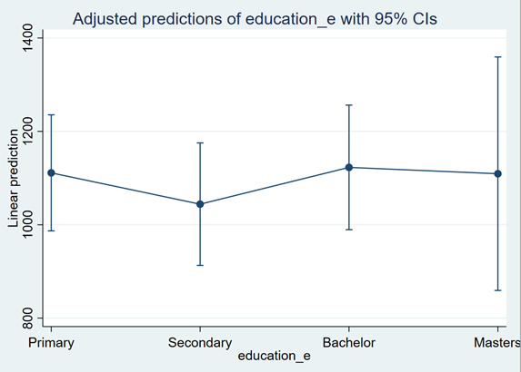
and then we can use marginsplot to graph these predict values:
marginsplot
We can also use bar charts instead of line charts. The command for bar charts is given below:
marginsplot, recast(bar)
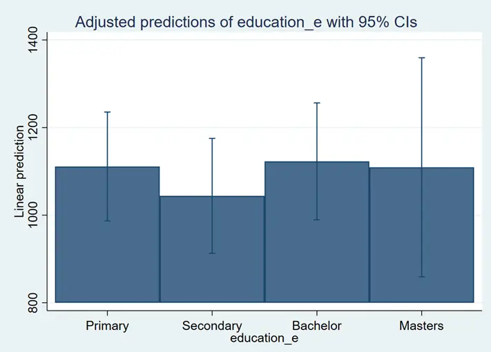
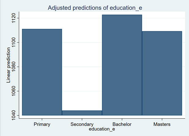
The blue lines on the bars are confidence intervals. We can remove them by using noci option:
marginsplot, recast(bar) noci
Changing Base in Categorical Regression
We can also choose the base or reference category of our own choice. For example, we want to use secondary education as a base, which is labelled 2, instead of primary. Then, in that case, we will use the below command:
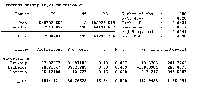
regress salary ib(2).education_e
The regression command will remain the same. Only the “i” will be replaced with the “ib”; within the parentheses, we will write the label we want to use. On executing the above, the secondary label (label = 2) will be used as the base.
To see the results with the base and other categories, use the below command with the allbaselevels option:
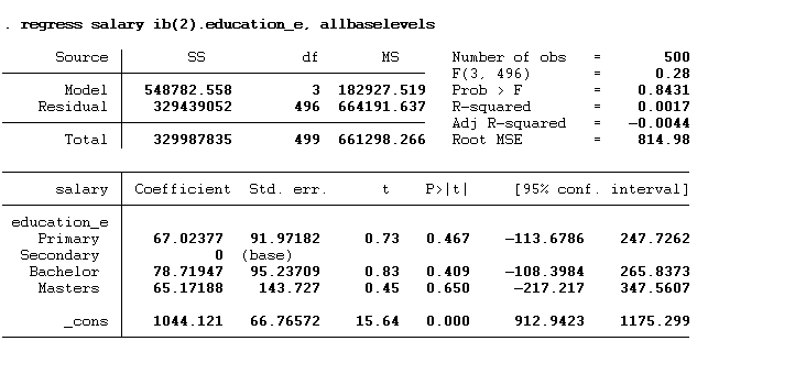
regress salary ib(2).education_e, allbaselevels
We can also write this command as given below:
regress salary ib2.education_e
Instead of providing specific value labels we can specify first, last or the category with highest frequency using following command:
regress salary ib(first).education_e regress salary ib(last).education_e regress salary ib(frequent).education_e
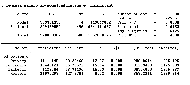
Lastly, if we want to use none of the categories as a base, then the command will be:
regress salary ib(none).education_e, noconstant
Remember to add the noconstant option at the end of the command; otherwise, you will face a dummy trap.
We can also change the base permanently in the Stata using the below command:
fvset base first education_e
fvset is the command to set the base category. The “base” in the command indicates that we are about to specify the base or reference level for the variable. “first” is the level that we are setting as the base. In this case, we are setting the “first” category as the base level. education_e is the variable for which you’re setting the base level.
Selecting Levels
It is also possible in Stata to add specific categories in the model. The command is given below:
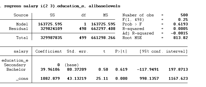
regress salary i(2 3).education_e, allbaselevels
In the above command, we tell Stata to use 2nd and 3rd categories only.
We can also set the range (1/3) as shown in the below command:
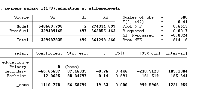
regress salary i(1/3).education_e, allbaselevels
We can also omit specific categories using “o” instead of “i” with a categorical variable (education_e), as shown in the below command:
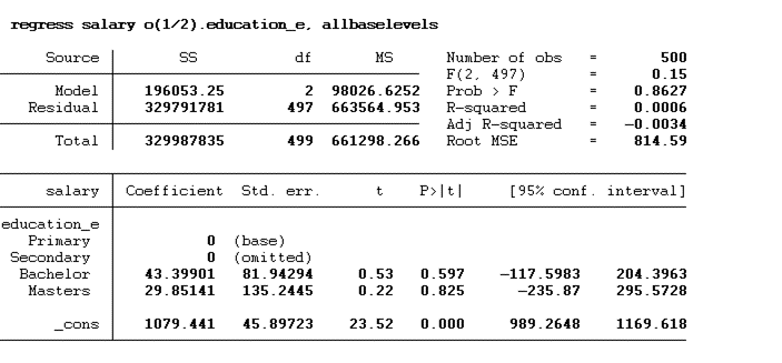
regress salary o(1/2).education_e, allbaselevels
Multiple Categorical Variables in Regression
We can also add two categorical variables in a regression, as shown below command:
regress salary i.gender_e i.education_e
The results are shown below:
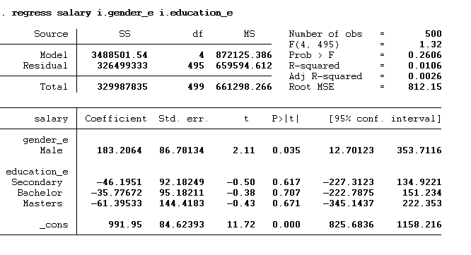
Now, we have two categorical variables, so this constant represents the predicted salary for both the omitted categories i.e. for the female with primary level of education. This constant value can be interpreted as the female having primary education on average earning 991.95 dollars. The rest of the interpretation will remain the same. The male would earn 183.206 dollars more than the female. Similarly, the individual with secondary education, bachelor’s and master’s would earn 46.195 dollars, 35.777 dollars and 61.395 dollars less than primary education individuals.
Margin Plot
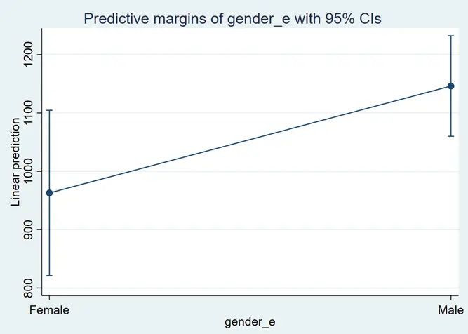
However, the margin plots for both categorical variables will be created separately using the following:
margins gender_e marginsplot
margins education_e marginsplot
Categorical and Continuous Variable in Regression
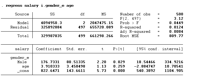
Having both categorical and continuous variables in the regression is also possible. Let’s assume we want to see the impact of age and gender on the salary. The below command will be used:
regress salary i.gender_e age
Margin Plot
We can also make the margin plot for the continuous variable. The command is given below:
margin , at(age=35)
First, we will write the command margin; after the comma, we have to specify an age at which we want to predict the value. Therefore, after comma, we will use at option and specify the variable’s name with its value within the parenthesis. The results are shown below:
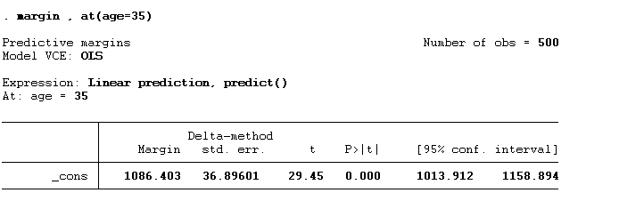
The results can be interpreted as the person having the age of 35 would earn 1086.403 dollars.
We can also predict the value for the range of age as shown in the below command:
margin , at(age=(20/55))
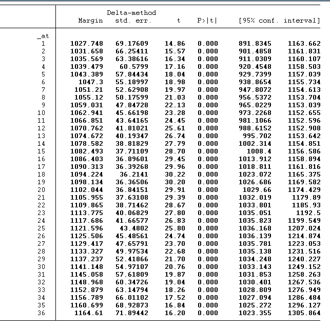
We can use the below command to create the margin plot of the above values. The command can be used for a line plot with a confidence interval.
marginsplot , noci recast(line)
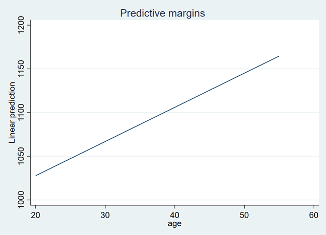
The line plot represents the beta coefficient of the age range from 20 to 55. According to the above graph, the average salary increases with increasing age.
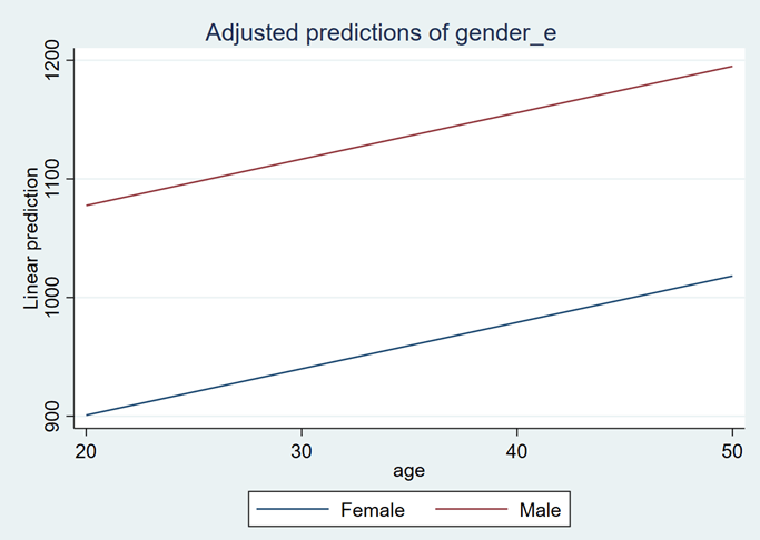
We can also look at the margin plot for the categorical and continuous variables. The command is given below:
margin gender_e, at(age=(20/55)) marginsplot , noci recast(line)
We will simply add the categorical variable name with the margin command and before the comma.
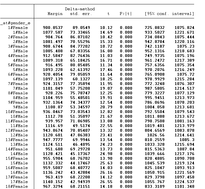
The predicted value for females and males of each age has been estimated. In the above figure, 1 represents the age of 20, 2 illustrates the age of 21 and so on. The graph is shown below:
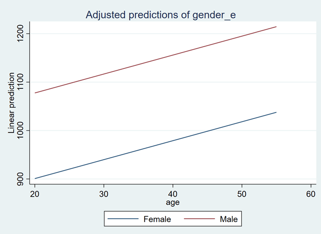
The blue line represents the female salaries, and the red represents male salaries in different age ranges. According to this age, the female earns less than the male at any age level.
We can also increment the age value to 10 using the command below:
Margin gender_e, at(age=(20(10)55))
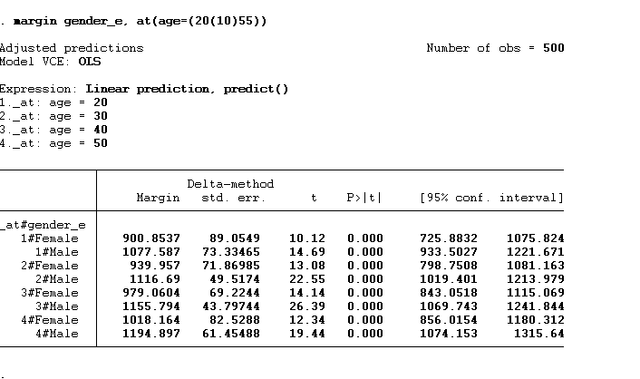
So, we will not get so many values when we do that. We will get values for 20, 30, 40 and 50. The graph will remain almost similar.