
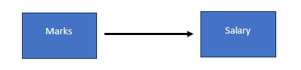
In our previous articles, we began understanding categorical variables, starting with the basics. We unraveled the importance of these variables in regression models and laid the groundwork for transforming categorical variables into a format suitable for quantitative analysis. We already looked into the regression with single categorical and multiple categorical variables. This article will shed light on the interaction between the categorical and continuous variables. We will use the same dataset we used in the previous two articles:
Download Example File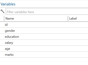
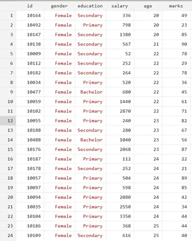
The dataset contains two categorical variables, gender (male and female) and education (Bachelor, Master, Primary, and Secondary), and three continuous variables, salary, age, and marks. Remember, before proceeding to the regression, we must encode the gender variable to convert qualitative into quantitative categories. The commands are given below:
encode gender, generate(gender_e) encode education, generate (education_e)
Interaction between categorical and continuous variable
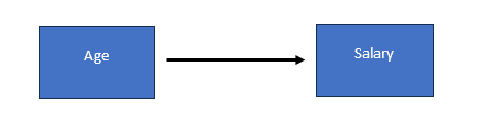
Suppose we have three variables, age, gender, and salary. Age is the independent variable, salary is the dependent variable, and gender is the moderating variable. A moderating variable affects the direction or strength of the relationship between an independent and a dependent variable. If we look at age and salary, we might hypothesize that age impact the salary.
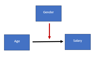
Now, if we bring gender into the mix as a moderating variable, it means that the image of age on salary might differ based on gender..
To see the impact of the moderating variable, we multiply the age by gender, this variable will known as the interaction term between age and gender. If the interaction term is significant, we conclude that there is moderating role of gender. The command of the regression to execute this concept in Stata is given below:
regress salary i.gender_e c.age i.gender_e#c.age
Remember that we have to include both the main effect and the interaction term. So we will include both the gender and age separately as well as the multiplication term of age and gender. As gender is categorical so we have used i. prefix for gender, age is continuous therefore, we have used c. prefix. Lastly, i.gender_e#c.age is the interaction term, we don’t need to create a variable that would be a multiplicative term of both these variables, rather in Stata we can use # sign for this purpose.
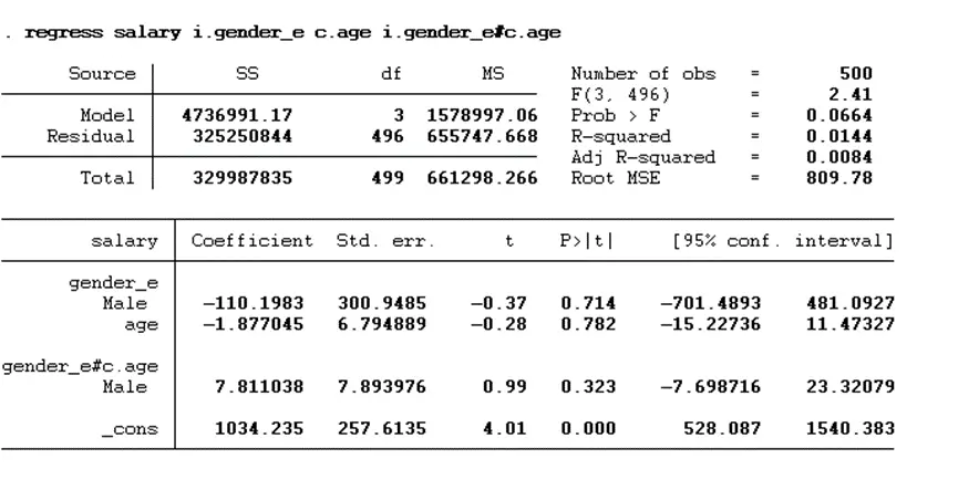
If the p-value of the interaction variable is less than 0.05, then we conclude that moderation exists. However, as per the above results, the p-value of the interaction terms of age and gender is greater than 0.05, which indicates that the moderation does not exist. If we want to make the command short, then the below command can be used:
regress salary i.gender_e##c.age
The real difference between these two commands is their presentation, output, or function. The first command specifies each term individually, while the second command uses Stata’s shorthand to include both the main effects and the interaction in one go. The results of the regression will be the same for both commands. This double-hash (##) is a shorthand in Stata that simultaneously includes the main effects (dummy variables for gender_e and the continuous age variable) and their interaction.
For ease of interpretation, we can make margin plot using below command:
margins gender_e, at(age=(20(1)55))
margins is the command which tells Stata that you want to compute the margins (predicted values or marginal effects) for each category or level within the “gender_e” variable. If “gender_e” is a binary categorical variable (e.g., 0 for male and 1 for female), then Stata will compute the margins for both male and female categories. at(age=(20(1)55)) specify the values of the “age” variable for which we want these predictions or marginal effects. age=(20(1)55) notation means we are interested in computing predictions/marginal effects for the “age” variable from 20 to 55, increasing in single units (increments of 1). So, Stata will compute these values for ages 20, 21, 22, up to 55.
marginsplot ,noci recast(line)
marginsplot is the command, noci, and recast(line) options to tell Stata that we don’t need a confidence interval and want to create a line chart.
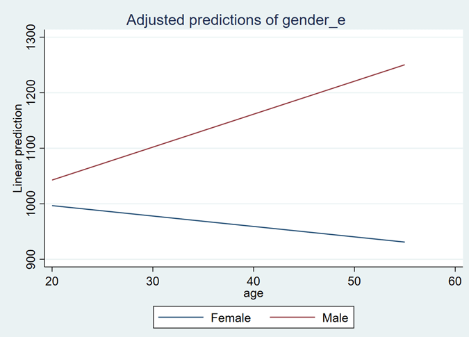
On the x-axis, we have age, and on the y-axis, we have predicted values of salary. The graph shows two lines, one for females and the other for males. So, this graph represents the impact of age on the salary for females and males. According to the graph trend, the female’s salary reduces with an increase in age while the male’s salary increases with an increase in age (Don’t worry this is hypothetical data and have nothing to do with real world).
Interaction between two categorical variables
Suppose we have three variables, age, gender, and salary. Education is the independent variable, salary is the dependent variable, and gender is the moderating variable. If we just look at education and salary, we might hypothesize that there is an impact of education on salary.
Now, if we bring gender into the mix as a moderating variable, it means that the relationship between education and salary might differ based on gender. In this case, the hypothesis will be that the impact of education on the salary varies based on gender.
The command to test this hypothesis on the Stata is given below:
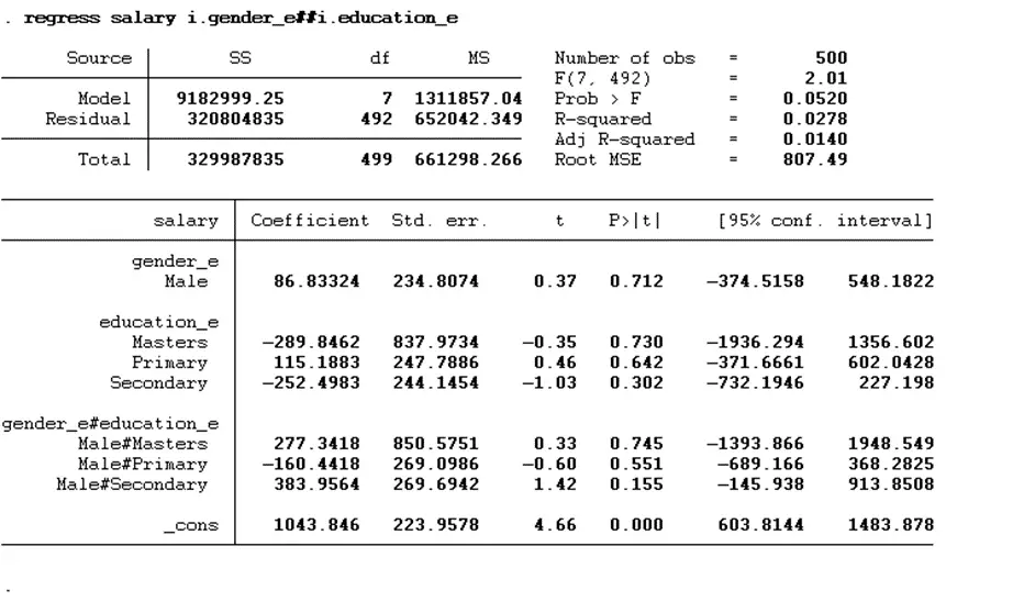
regress salary i.gender_e##i.education_e
The command used to execute the regression is regress, salary is the dependent variable, i.gender_e is the moderating variable, and i.education_e is the independent variable. The double-hash (##) operator between the moderating and independent variable instructs Stata to include the main effects of the two categorical variables (gender and education level) and their interaction term in the model.
To better understand the results, we will create a margin plot using the following:
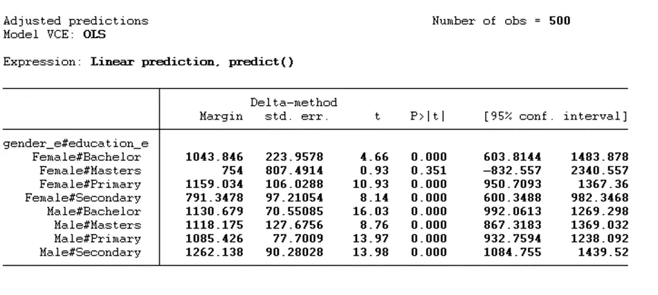
margins i.gender_e#i.education_e
margins is the command, and i.gender_e#i.education_e are the interaction terms of moderating and independent variables. This will provide the predicted value for females and males at different education levels.
To plot these values in a graph, the below command can be used:
marginsplot
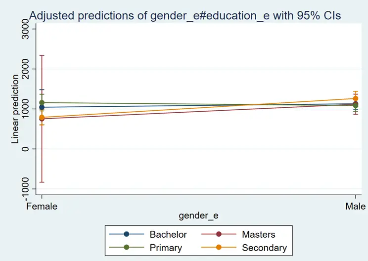
This graph is quite difficult to understand. We can understand this easier if we have this education on the x-axis. This command for that is given below:
marginsplot, xdimension(education_e) recast(line) noci
xdimension(education_e) specifies that the x-axis of the plot should represent different levels or values of the variable “education_e”. The plot will show how the predicted outcome or marginal effect varies across these levels. The recast(line) option tells Stata to produce a line plot instead of the default. noci stands for “no confidence interval.” It instructs Stata not to plot the confidence intervals around the predicted values or marginal effects.
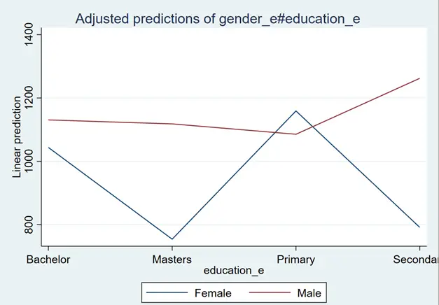
The blue line represents the impact of education on salary for females, and the red line represents the impact of education on salary for males. The salary of a female with a secondary, bachelor’s degree, and master’s degree would be less than that of a male with a secondary, bachelor’s degree, and master’s degree. In comparison, females with primary education would earn more than males.
Interaction between two continuous variables
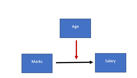
Suppose we have three variables, marks, age, and salary. Marks are the independent variable, salary is the dependent variable, and age is the moderating variable. If we look at marks and salary, we might hypothesize that marks impact the salary.
If we bring age into the mix as a moderating variable, the relationship between marks and salary might differ based on the individual’s age. In this case, the hypothesis will be that the impact of marks on the salary varies on the base of the age of the individual.
To investigate the impact of this moderate, we will calculate the interaction term between marks and age similarly we did before. The command is given below:
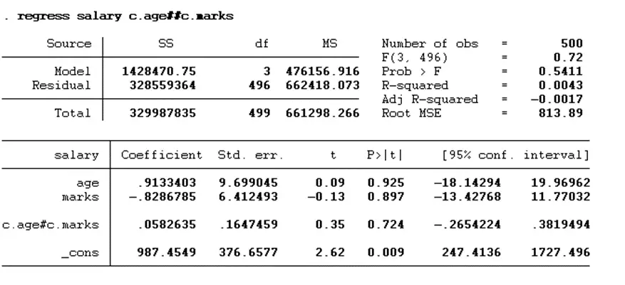
regress salary c.age##c.marks
In the above command, regress is the command for regression, salary is the dependent variable, age is the moderating variable, and marks is the independent variable. The double-hash (##) operator between the moderating and independent variable instructs Stata to include the main effects of the two continuous variables (age and marks) and their interaction term in the model. The results are presented below:
To better understand, we will make the margin plot using the below commands:
margins, at(marks=(20(5)90) age=(20(10)55))
margins is the command to get predicted values or marginal effects. at is the option that specifies the values of the independent variables at which we want to compute these predictions or marginal effects. marks= (20(5)90) is the notation indicates that we want predictions or marginal effects for the variable “marks” at values from 20 to 90 in increments of 5. So, it will compute predictions/marginal effects for marks at 20, 25, 30, up to 90. age= (20(10)55) is the same, but for the variable “age,” we are asking Stata to compute predictions or marginal effects at values starting from 20 to 55 in increments of 10. This means predictions/marginal effects will be computed for age at 20, 30, 40, 50, and 55.
marginsplot, recast(line) noci
marginsplot is the primary command, instructing Stata to produce a plot based on results from a prior margins command. The recast(line) option tells Stata to produce a line plot instead of the default. noci stands for “no confidence interval.” It instructs Stata not to plot the confidence intervals around the predicted values or marginal effects.
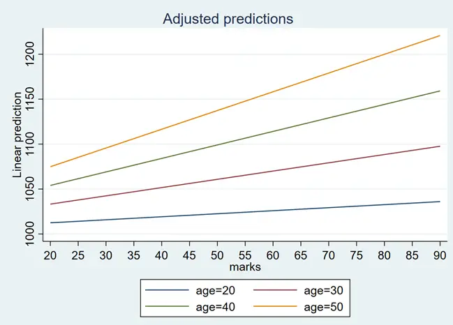
The above graph represents the impact of marks on the salary at different age intervals. The graph can be interpreted as if the individual is at the lowest age, then his/her salary would change a lot with an increase in marks. However, with the increase in age, the impact of marks with increase on the salary. To change the dimension, for example we want age on a-axis then we can use below command for margin plot:
marginsplot, recast(line) xdimension(age) noci
marginsplot is the primary command, instructing Stata to produce a plot based on results from a prior margins command. The recast(line) option tells Stata to produce a line plot instead of the default. xdimension(age) specifies that the x-axis of the plot should represent different levels or values of the variable “age”. noci stands for “no confidence interval”. It instructs Stata not to plot the confidence intervals around the predicted values or marginal effects.
