In our previous article, we embarked on a journey through categorical variables. From foundational principles, we highlighted their role in regression models and emphasized techniques to adapt these variables for quantitative studies. In this fourth article, we will discuss three-way interactions, enriching our understanding and decoding their significance. The dataset we use in this study includes the following variables:
Download Example File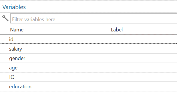
Three Way Interaction
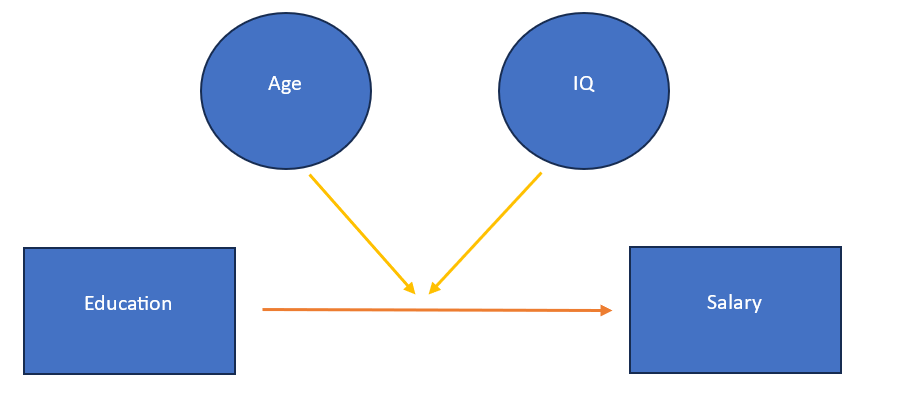
Three-way interactions build upon the concepts we’ve touched upon in our previous article related to Two-way interaction. The distinguishing feature here is that we examine the influence of two moderating variables on the relationship between the independent and dependent variables instead of one. For example, we want to see the impact of education on salary, considering that this relationship is moderated by the two moderating variables, gender and IQ. It can also be explained as the impact of education on salary differs for different genders and levels of IQ.
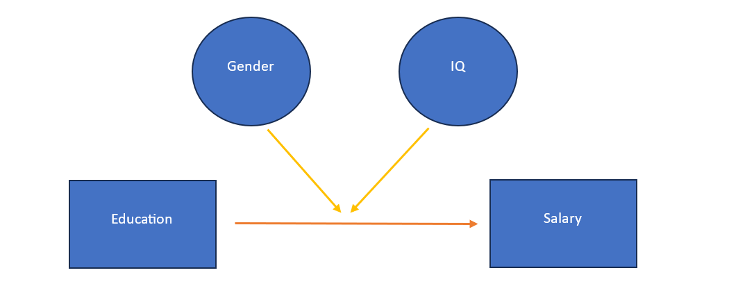
The above example includes one categorical variable (gender) and two continuous variables (education and IQ), in addition to the dependent variable. In this case, one variable out of three interacting variables is categorical. It is also possible to have all the continuous variables as shown in below figure:
In this article, we will focus on models with one categorical variable in a three-way interaction variable and then delve into those exclusively containing all three continuous variables (i.e. the independent and moderators are continuous). In the three-way interaction, the equation looks somewhat like this:
Salary = b0 + b1X + b2M1 + b3M2 + b4XM1 + b5XM2 + b6M1M2 + b7XM1M2
Here, salary is the dependent variable, b0 is the constant, b1X is the independent variable, b2M1 is the first moderating variable, b3M2 is the second moderating variable, b4XM1 is the two-way interaction variable of the independent variable with the first moderating variable, b5XM2 is the two-way interaction variable of independent variable with the second moderating variable, B6M1M2 is another two-way interaction variable between the two moderating variables, and lastly b7XM1M2 is the three-way interaction variable between the independent variable and two moderating variables.
Three-Way Interaction between Categorical and Continuous Variables
Let’s move towards the regression command that includes two moderating variables, one categorical and one continuous. The command is given below:
regress salary i.gender##c.IQ##c.education
In the above command, i.gender##c.IQ##c.education includes main effects for gender, IQ, and education. Include interaction terms for gender and IQ, gender and education, and IQ and education. Also include a three-way interaction term for gender, IQ, and education. The empirical model of this example is given below:
salary = b0 + b1edu + b2gender + b3IQ + b4edu*gender +b5edu*IQ + b6gender*IQ + b7edu*gender*IQ
The results we get after execution of the above command are given below:
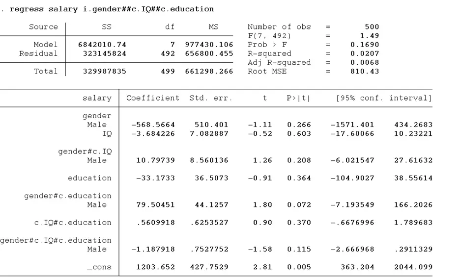
To conclude that the moderating impact is significant, it is just that the p-value < 0.05 of the variable gender#c.IQ#c.education. In the above example, the p-value> 0.05 means that there is no moderating impact of education and IQ on the relationship of gender with salary.
It’s quite difficult to interpret the above coefficient, but the margin plots can make it easy. So now we will make the margin plot using the below command:
margins gender, at(IQ==(20(5)50) education=(2(2)18))
We will use the margins command to generate margins and then name the categorical variable. at() option specifies the values of the variables at which the margins are to be evaluated for the continuous variables. In our example, it’s IQ and education. IQ== (20(5)50) tells Stata to compute margins at specific values of the ‘IQ’ variable. Specifically, we want predictions for IQs starting at 20, increasing by increments of 5, up to and including 50. This would predict IQ values of 20, 25, 30, …, 50. education= (2(2)18) Similarly, Stata calculates margins for ‘education’ starting at 2, increasing in steps of 2, up to and including 18. We are not particularly interested in margins, however, we need these margins to generate margins plot. Then, we will use the below command to generate the margin plot.
marginsplot,by(gender) noci
by(gender) option specifies that separate plots or lines should be generated for each level of the ‘gender’ variable. So, if ‘gender’ has two levels (e.g., male and female), we get two plot lines or sets of points, one for each gender. noci option stands for “no confidence interval”. By default, the margin plot will draw confidence bands around the predicted values to represent uncertainty. The noci option tells Stata not to display these confidence intervals, resulting in a cleaner plot focusing on the predicted values.
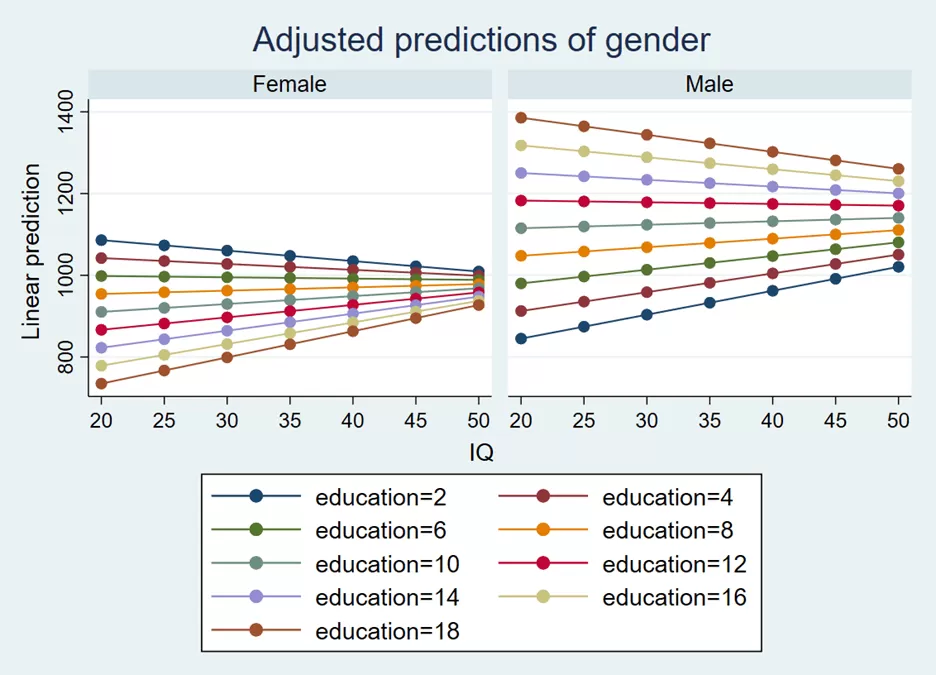
The above plot shows IQ on x-axis, however, from figure 1 we know that education is our independent variables and should be placed on x-axis. If we plot education on the x-axis, then we use the below command:
marginsplot,by(gender) noci xdimension(education)
xdimension(education) option sets ‘education’ as the x-axis of the plot. The predicted values (or adjusted means) will be plotted against the different levels or values of ‘education’ specified in the earlier margins command.
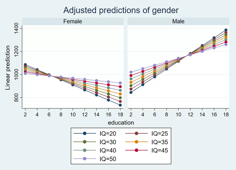
The coloured lines on the graphs show the different levels of IQ’s. This graph explains that the impact of education is different for females and males. When the education of males increases, the salary increases. Furthermore, the impact of education on salary is lowest at the lowest level of IQ (i.e. IQ=20), but after a certain level of education say 12 standard, the slope/impact of education on salary is highest for the lowest level of IQ (i.e. IQ==20). Note: Don’t worry this is hypothetical data and does not have anything to do with real word, so keep on increasing your IQ and education 😊.
Three-Way Interaction with All Continuous variables
In this example, we are using all continuous variables as shown in Figure 2. The command is given below:
regress salary c.edu##c.IQ##c.age
The command is the same; only gender, a categorical variable, is replaced with age, a continuous variable. The empirical model of this example is given below:
salary = b0 + b1edu + b2age + b3IQ + b4edu*age +b5edu*IQ + b6age*IQ + b7edu*age*IQ
The results are given below:
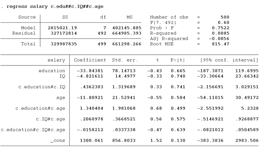
Constructing margin plots becomes complex with three-way interactions, especially when all variables are continuous. To navigate this complexity, we often adopt threshold values for the continuous variables in our model, namely IQ and age. We will identify the upper and lower bounds for age and IQ. Essentially, we are transforming these continuous variables into categorical variables. We will subtract the standard deviation from the mean to get high and low values. Firstly, we will use the summarise command below to get the mean and standard deviation. Let’s do it for the age variable first.
summarize age
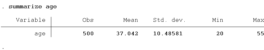
Now, we will use the global macro to calculate values by adding and subtracting the standard deviation from the mean. This command will produce two variables: the high (h) value and the low (l) value. However, these variables won’t be visible within our dataset. These variables will be stored in the internal memory of the Stata. The commands are given below:
global h=37.042+10.48581 global l=37.042-10.48581
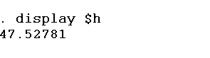
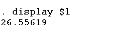
To see these values, we can use the display command and $ sign with high (h) and low (l) variables.
display $h display $l
This method has potential pitfalls and we have to input the values manually, which cannot be automated if you change the dataset, therefore a more appropriate approach is to automate this process, using following commands. Let’s execute the summarize command for again once again:
summarize age
This summary command stores different scalars shown below:
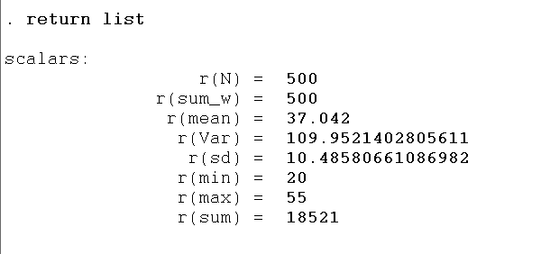
Then, we will use the global macro again. The command is given below:
global HighM1=r(mean)+r(sd) global LowM1=r(mean)-r(sd)
HighM1 is the name of the macro, equal to the mean plus standard deviation, and LowM1 is the name of the macro, equal to the mean less standard deviation.
We will repeat this process for the IQ variable. The commands are given below:
summarize IQ global HighM2=r(mean)+r(sd) global LowM2=r(mean)-r(sd)
Now, we are able to generate margins.
margins, at(education=(2(3)18) age=($HighM1 $LowM1) IQ=($HighM2 $LowM2))
education=(2(3)18) indicates that margins are to be computed for the ‘education’ variable starting at a value of 2, increasing in increments of 3, up to 18. So, we are looking at education levels of 2, 5, 8, …, 18. age=($HighM1 $LowM1) is for margins to be computed at specific values of ‘age’, which have been stored in the global macros HighM1 and LowM1. Using the dollar sign, $ allows us to reference the values stored in these global macros. IQ=($HighM2 $LowM2) is similar to the ‘IQ’ variable, margins are being computed for values stored in the global macros HighM2 and LowM2. The results are given below:
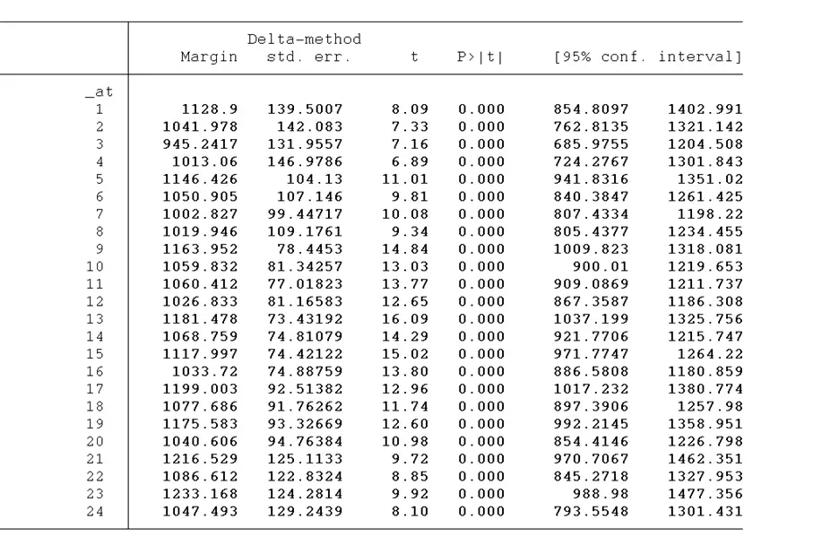
After getting the margin, we will plot them in the graph using the below command:
marginsplot, recast(line) noci
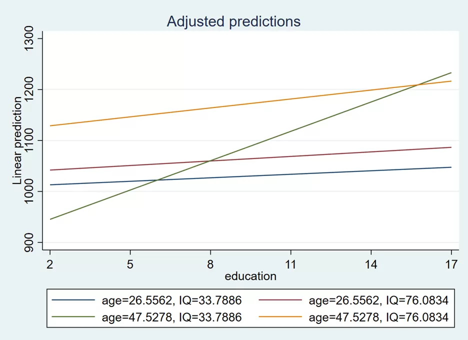
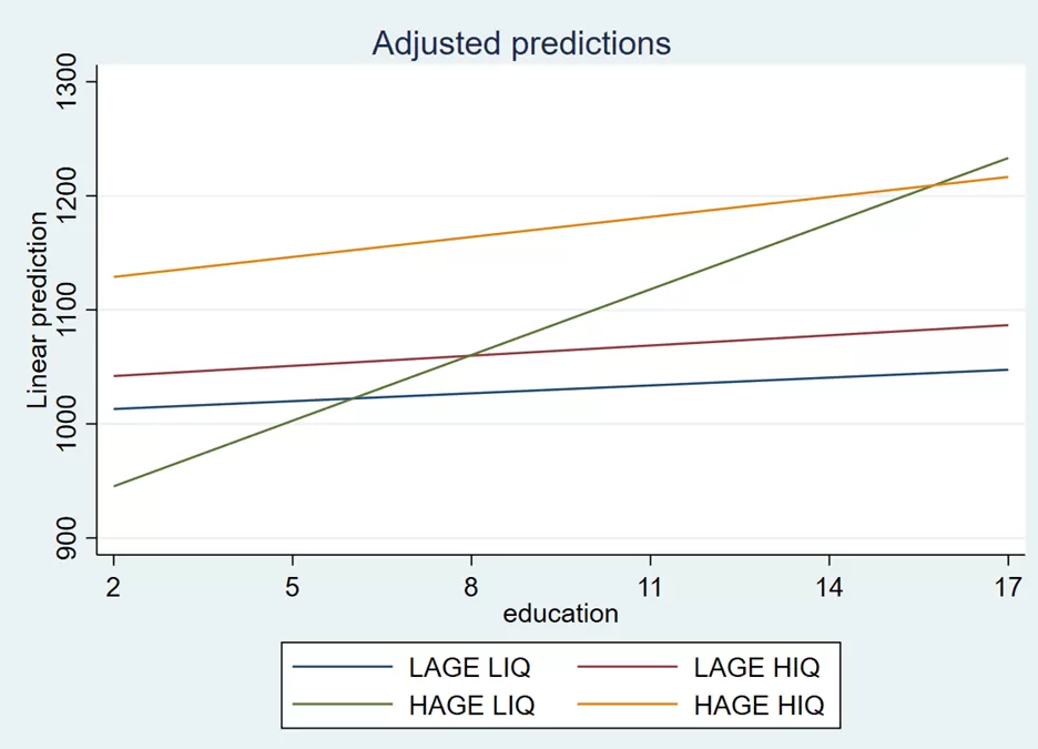
In the above graph, the blue line represents low age and low IQ, the red line represents low age and high IQ, the green line represents high age and low IQ, and the yellow line represents high age and high IQ. We can also label this combination using the below command:
marginsplot, recast(line) noci legend(order(1 "LAGE LIQ" 2 "LAGE HIQ" 3 "HAGE LIQ" 4 "HAGE HIQ"))
legend(order(1 “LAGE LIQ” 2 “LAGE HIQ” 3 “HAGE LIQ” 4 “HAGE HIQ”)) part of the command deals with the legend of the plot. It specifies the order and labels for the legend entries. It seems that there are four categories labelled “LAGE LIQ,” “LAGE HIQ,” “HAGE LIQ,” and “HAGE HIQ,” and they are assigned the order of 1, 2, 3, and 4, respectively. The graph is given below: