
Exploring the various data types in Stata is crucial for effective data management and data analysis. In Stata, there are four main data types including integers, decimal numbers, strings and dates. A command
help datatype
will open this window that gives you an in depth analysis of the characteristics of all these data types.
Download Example File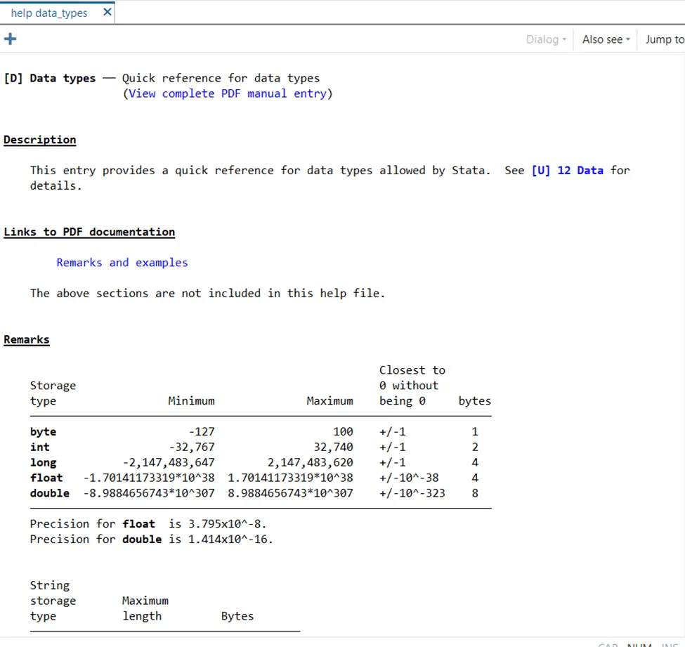
Join us as we delve into each data type to comprehend its properties along with learning about data manipulation techniques that help optimize our Stata workflow.
Integers:
First up, we have integers. Stata classifies integers into three categories, namely, byte, integer, and long. Each type of integer can accommodate a specific and distinct range of integer values. For example, a byte can store values from -127 to 100, while an integer may hold values within a more extensive range i.e. -32,767 to 32,740.
Decimal Numbers:
In Stata, Decimal Numbers are represented by two types, namely float and double. Both of these types cater to different precision levels. Float accommodates single precision floating point numbers while double decimal numbers store double precision floating point numbers.
Strings:
Whenever you need to store textured data, Strings are your friend. String variables can be identified by different labels that indicate the maximum number of characters they can hold, like str1, str2, str3 etcetera. For instance, str50 can hold up to 50 characters!
Dates:
As the name rightfully suggests, date data types are specifically designed to store temporal data. They are significant for time series analysis and can manage various date formats.
Generating Variables with Specified Data Types:
The ‘generate’ command in Stata allows us to create variables with designated data types. For the sake of an example, let us generate a number with the string data type. The command for this specific example is as follows,
generate str50 number=”123”
Let us also generate a variable, for instance called ‘double’, and let us make it equal to mpg through this command
gen double mpg2=mpg
Upon both of these command, you can browse your data editor that would show data in this form.
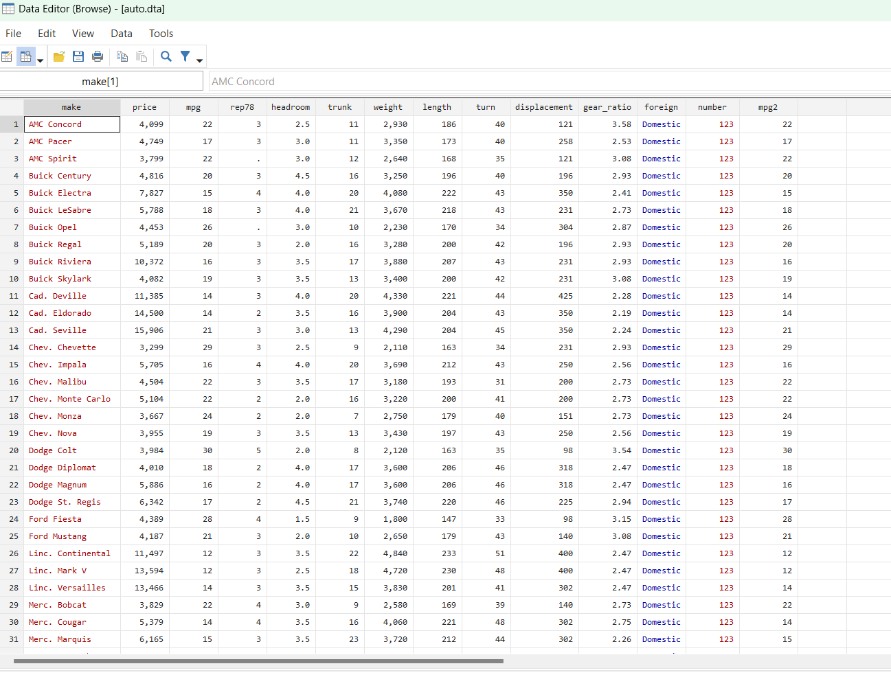
Please also note that the mpg 2 has a double data type.
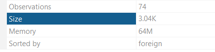
In the far right corner, you can see the size of your data file too. It would show something like this,
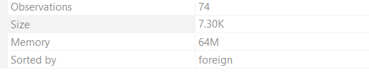
As we increase the capacity, it would directly reflect in the size of the data set: increasing it. To manage the size of the data set, we have another command to master.
Managing Data Sizes with the ‘Compress’ command:
Data sizes need to be critically considered while working with large data sets. Here, the
compress
Compress command comes in handy. This command is a powerful tool that helps minimizing storage requirements. By optimizing the data sets, it significantly reduces the data set size while also ensuring that the essential information is rightly retained.
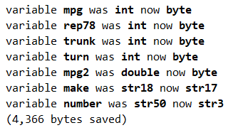
To explain further, executing this command on your dataset can lead to substantial space reduction by converting variables into more space-efficient data types. Memory efficiency can be particularly enhanced by this beneficial trick. As we run this command, it has effectively reduced the size of our data set to half, by converting different variables, as shown in the illustrations below. For example, mpg was converted from integer to byte. This step is repeated on several variables to make them more space efficient. Note that the variable ‘number’ has been changed from str50 to str3 to save space. Although it originally had the capability to hold characters up to 50, it was only holding 3 characters. Thus it was reduced to the maximum numbers of characters it had to be space efficient.
Changing Data Types with ‘Recast’ Command:
Moving on, The ‘recast’ command helps to change the storage types too. It enables us to alter the data types of our variables.
For the sake of explanation, a command
recast double price
can convert the price from current data type to the ‘double’ data type. It would show in the Properties of the variables as such,
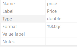
However, it is important to remember that the ‘recast’ command works best with numeric variables. It is helpful in converting numeric variables between various numeric types and altering the length of string variables. Yet, it can not convert numeric data to string or string to numeric data. If you wish to do convert numeric data into string or vice versa, Stata provides commands like ‘encode’, ‘decode’, ‘destring’ and ‘tostring’.
Understanding and choosing appropriate data types in Stata plays a pivotal role in efficient data analysis and storage. You can make informed decisions by comprehending the differences and distinctions between integer, decimal, string and data types. The ‘generate’ command facilitates the creation of variables with their specific types. The ‘compress’ command optimizes and reduces memory usage. The ‘recast’ command works wonders for transforming variable data types. Armed with these insights, you will surely be better equipped to manipulate data efficiently in Stata, enhancing your analytical capabilities and workflow efficiency.