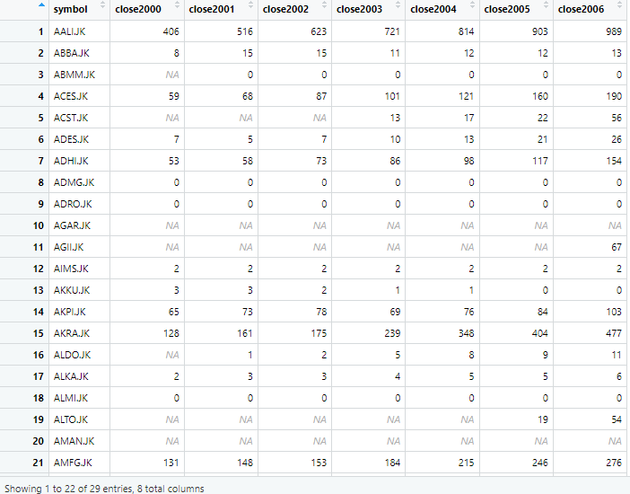
Reshape in R is when data is transformed from one form to another. The data can take a long form or wide form. In the wide form, each row represents a unique entity and each variable is spread across multiple columns. For example, consider a data set of a company, having stock prices for different years. In this data set, there is no separate or unique column for each variable. This type of format is used when data is aggregated or summarized, each variable represents a specific measurement. Thus, the wide format is useful for quick summaries or comparison between different entities.
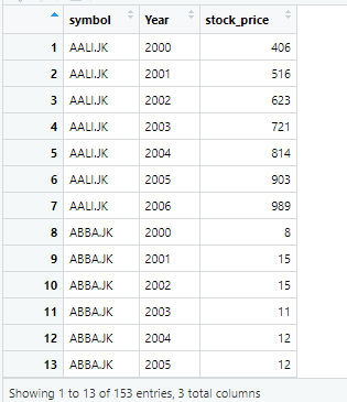
In long form data, also known as tidy format, each row represents a unique observation and each variable has it own column. For example, consider again the data set of a company, having stock prices of different years. The data shown below has a separate column for both variables, i.e. stock prices and year. This type of format is often used for data analysis, data manipulation and modeling.
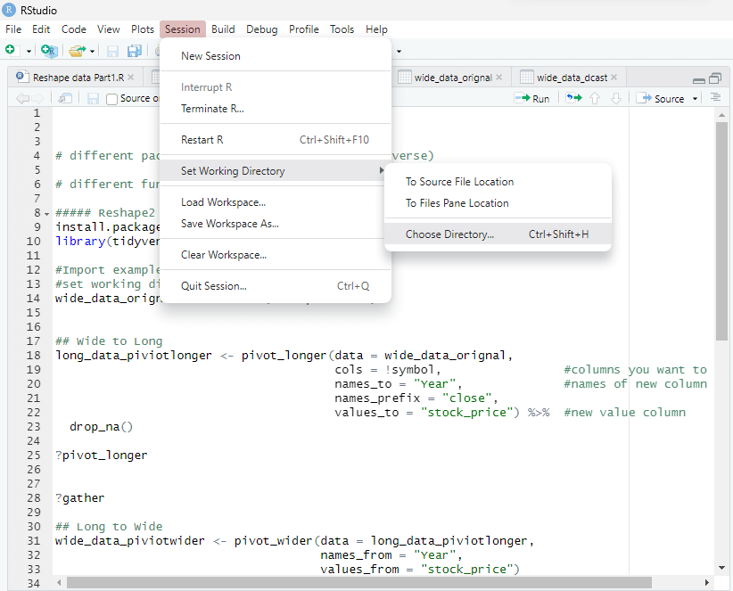
These different type of data formats can be transformed, or we can reshape it in R from one format to the other. Before we start reshaping the data, first set the working directory of R, by using session option in window bar in R, as shown below. The working directory should be set where your file, that you want to reshape in R, is saved.
Reshaping data from wide to long format
There are two widely used packages that reshape the data in R. These packages are named as tidyverse and reshape2. These packages aren’t pre-installed in R. So to use these packages, we first need to install these packages in R. To install these packages, we use following command in R.
install.packages(tidyverse)
Once the package, that reshape data in R has been installed in R, the next step is to activate the package. To activate the package, usually known as library, we run the following command in R.
library(tidyverse)
Remember that, even you have installed package in R already, you need to activate the package every time before using the package.
Once the package has been activated, next step is to load data from the working directory. To set or change working directory, go to session in R studio and change or set working directory, as explained earlier.
Once the directory has been set, now you can import the data set using the file name of data set by which it is saved. In this case, the data set is imported by using following command
wide_data_orignal <- read.csv("example1.csv") The data has 29 observations and 8 variables, which can be seen from the environment window in R, as shown below.
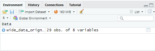
If we click on wide_data_origin in environment window, data can be visualized as below

In above command, data set has been saved by the name example1. Once the data has been imported, now convert the data from wide form to long form. To do this, we use the pivot_longer command in R. The pivot command is used along with many other options to reshape data in R, in wide form to long form, as show below.
pivot_longer(data = wide_data_orignal, cols = !symbol, names_to = "Year", values_to = "stock_price")
Here pivot_longer as the name suggests is used to reshape data in R from wide format to long format. It requires several other parameters with it too. First, we need to provide the data set that is required to be converted, which is wide_data _original here. Next, we specify columns that we want to reshape. To do so, we use exclamation mark with a certain column. Exclamation mark (!) in R means “not”, so if we add exclamation mark with a column name, R will not include that column while reshaping data. In this case, symbol is the column that we don’t want to be reshaped. So when we add exclamation mark with column “symbol” R will select all other columns except symbol column while reshaping data. Thus, we used the exclamation mark in R to exclude the symbols’ column in reshaping data.
Additionally, we need to specify the names of the new column that will be generated from reshaping data from wide to long. As in wide format, the columns are years e.g. 2000, 2001 and so on, we name the new column “year”. Lastly, we specify the name of the new column that will hold the values. Since we know these values represent stock prices, we create a new column called “stock_price” to store them.
The data generated in long format has 203 observations of 3 variables. You can check this detail of variables and observations from environment window in R.
Once you click on the data in environment window, data is visualized as below
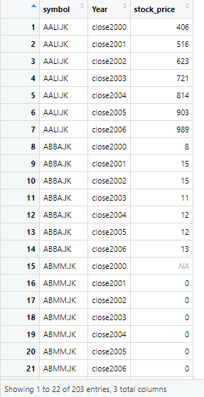
The data is same as previous data, just the format is changed from wide to long. However, there is a word “close” written along with years. That doesn’t seem suitable, so we remove the word close from years. Now to remove word close which is used as a prefix in year column, we use the following command
pivot_longer(data = wide_data_orignal, cols = !symbol, names_to = "Year", names_prefix = "close", values_to = "stock_price")
Now if we look at the year column, it doesn’t have close as prefix with years and data is cleaned now. However, there is still an issue. In stock price column, there are certain values that are missing. These missing values are present in the form of NA in R, as shown below
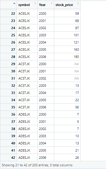
To deal with these missing values, we use the drop option in R, which will drop these missing values.
long_data_piviot longer <- pivot_longer(data = wide_data_orignal, cols = !symbol, names_to = "Year", names_prefix = "close", values_to = "stock_price") %>% drop_na()
In above command, we instruct the data to remove missing values represented as NA by using drop_na() option. Once you execute the above command, the missing values are dropped and data has now 153 observations of 3 variables. Now, data looks like as following, i.e. it doesn’t contain any missing values.

Although it seems easier to read stuff related to R, doing R actually takes time and practice. If in any task related to R, you have certain confusions about how this command works, you can use the question mark ? sign with the command to get help from R related to that specific command. R will help by providing documentation of that specific package or command.
For instance, if you are confused about certain functions in pivot_longer command, you can use the question mark with the command to get help from R. The command will look like this
?pivot_longer
R will provide following explanation for the pivot_longer command, explaining its functions and usage etc.
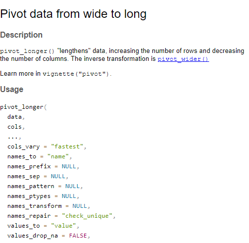
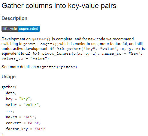
The pivot longer function in earlier versions of tidyverse package was called as gather, so pivot longer basically replaced gather in tidyverse. So if we are curious enough to know about the gather command, we use the question mark with gather to know about this command. The command used will be
?gather
So R shows that gather command is superseded and is currently replaced by pivot_longer. The gather command is thus no longer in use or will be of any help to convert data from wide to long format. The R help for gather is shown below
Converting data from Long to Wide Format
Now we convert data from long to wide format. Remember that, we said earlier in wide format, each row represents a unique entity and each variable is spread across multiple columns. So Each variable doesn’t have a unique column in Wide format. We convert the data that we have in long format, having 153 observations of 3 variables.
The data that we have in long format has three variables named symbol, year and stock price. As now each year will have a separate column, the name of column will be taken from the respective year. For instance, the year 2001 will have a separate column, 2002 will have a separate column and so on. So the name of column will be taken from the variable whose observation is being used.
The command that we use for converting data from long to wide format is as follows
wide_data_piviotwider <- pivot_wider(data = long_data_piviotlonger, names_from = "Year", values_from = "stock_price")
The wide data generated has 29 observations of 3 variables. If we open the wide data from environment, the following data is shown
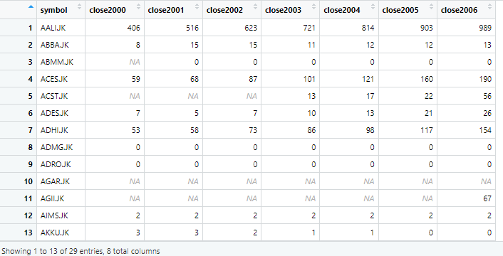
The above image shows that prefix closed is used again with the year column. To remove the prefix close, we use following command
# names_prefix = "close"
Now the issue has been fixed, and year column doesn’t have any prefix close with it.
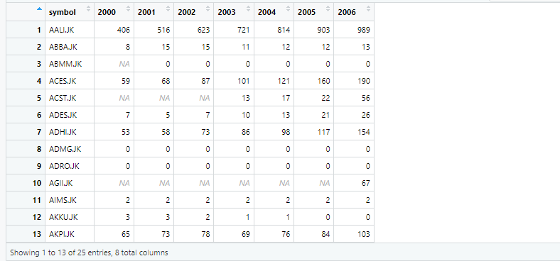
Now again, if we want any help related to pivot wider, we use the same method that we did earlier. The question mark sign with pivot_wider will open the help documentation from R.
?pivot_wider
It shows the command, explaining its functions and usage. You can scroll down further to get into more details of the command.
Just like pivot_longer replaced gather, pivot_wide replaced spread command. If we get help of spread, we can see that spread is superseded by pivot_wider and is no longer in use. So if you come across any old article of R, that uses gather or spread, remember that these commands are replaced.
?spread
In the above command that we used for converting data from longer to wider, we specified R from where to take values and from where to take name of the columns, however, even if we don’t specify R, and simply use the following command without parameters, it would generate similar results.
wide_data_piviotwider <- pivot_wider(long_data_piviotlonger, "Year", "stock_price")
Reshape2 Package to Reshape data in R
Other than tidyverse, there is another package named Reshape2 that is used for the reshaping data; convert data from long to wide format and vice versa. Reshape2 has two functions; melt and dcast.
The melt function is used to transform/reshape data from wide format to long format, so it is similar to pivot longer function. On the other hand, dcast function is used to convert data from long to wide format, so it resembles pivot wider function in tidyverse package.
To use reshape2 package, first we need to install this package. To install the package, use the following command
install.packages(reshape2)
Once the package is installed, next we run the library by using the following command
library(reshape2)
Next, we want to convert data from wide to long, so the melt function in reshape2 package will be used. The general syntax of melt function is melt(data, id.vars, variable.name, value.name). In this syntax, the data is that is required to be reshaped, id.vars is ID variable that can be used as identifier or as id( as the name suggests), id vars doesn’t change during transforming or reshaping data. The variable.name is the column name that stores the name of variables and lastly value.name is the name of column that stores the values of variables.
In this case, the data is original data that we used earlier, id.vars is symbol, name of column that stores variables is year and stock price is the name of column that stores values. The command will look like this
long_data_melt <- melt(data = wide_data_orignal,
id.vars = "symbol",
variable.name = "Year",
value.name = "stock_price")
The reshaped data will look like this
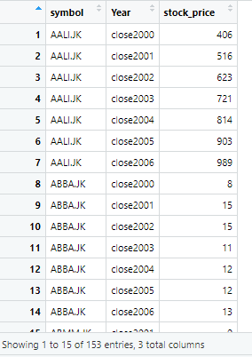
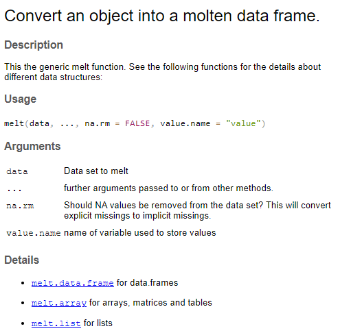
We can also get help from R regarding melt function using the following command
?melt
R will provide following documentation for the melt function
Now we want to convert data from long to wide format, using dcast function. The syntax of dcast is similar to pivot_wider which is dcast(data, formula). Here again, the data is that is required to be reshaped, formula shows the casting behavior, and can take the form of value.var column.variable, row.variable etc.
In our command, there is data in long form, that we want to reshape in wide form, years that were previously rows would now become separate columns and the values these years would take from. The command is shown as below
wide_data_dcast <- dcast(long_data_melt,
symbol ~ Year,
value.var = "stock_price"
)
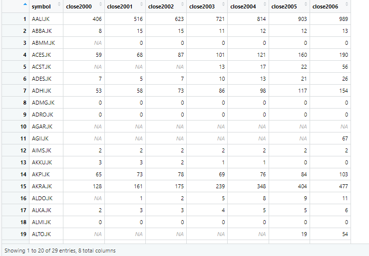
The data looks like as following
Just like other functions, documented help for dcast can be generated from R using following command
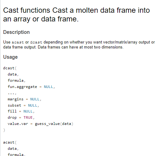
?dcast
