
This article details out the margin and marginal plots in Stata. The margins, in Stata, are referred to as a technique that is used to calculate the marginal effects of independent variables in models such as regression. Using margins, we can estimate the change in predicted values when one or more independent variable changes, keeping other variables constant.
Margin plot on the other hand is the graphical representation of marginal effects calculated using the technique of marginal command.
To demonstrate it further, let’s import a data set in stata, using the following command
webuse lbw
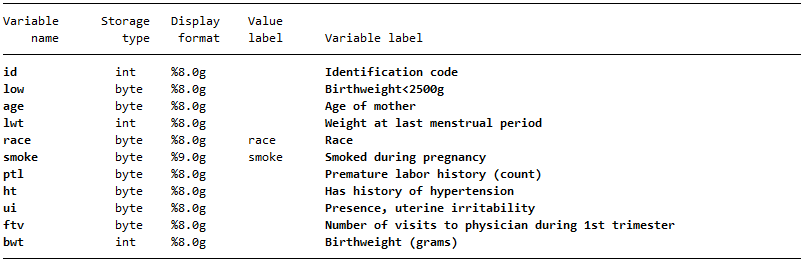
This data set contains information about the effect of smoker and non-smoker mothers on the weight of newborn babies. We first describe the data set to figure out what each variable is about. To describe the data set, use the following command
describe
This command generates the following results, that outlines the details of each variable in the data set.
Once we have the details of dataset, we can find the effect of smoking on birth weight of babies. To find the effect of smoking habits of mothers, on weight of the children, we regress birth weight on smoke using following command
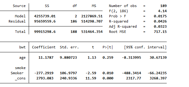
regress bwt age i.smoke
Note that, we used i.smoke variable in the regression. This is because smoke variable is categorical and to get margins for the smoke variable, we need to specify Stata about the categorical variable. The age variable is added additionally, which outlines the effect that how age of mother affects the birth weight of babies, depending on whether she smokes or not. Following regression results are generated from the above command
Margins in Stata
To get the marginal effects for the above regression, we use the following command
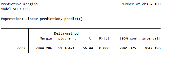
margins
This generates a table that predicts the expected birth weight of the babies, which is 2944.286 grams, based on the data set.
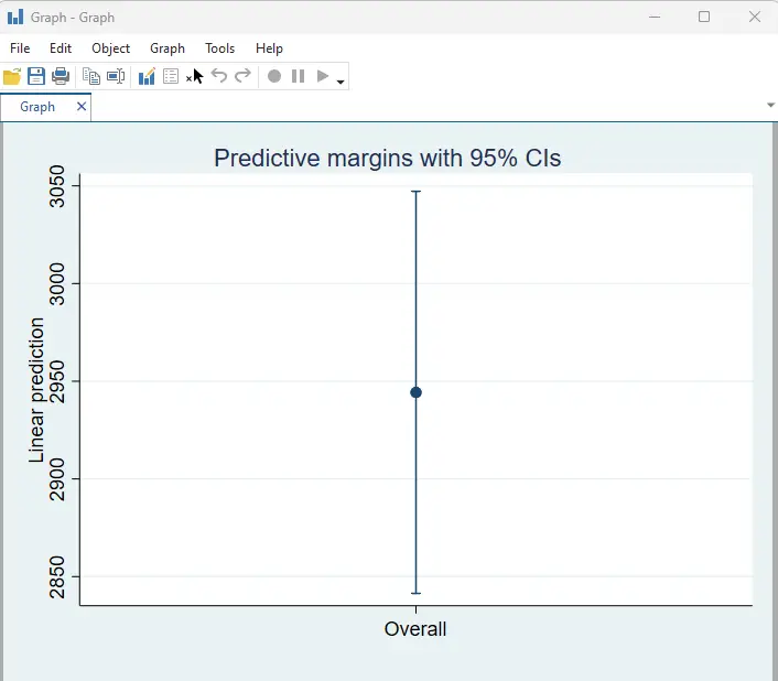
We can get the graphical representation of above margins. To get the visual representation of these margins, we use the following command to generate margins plot in Stata
marginsplot
The following marginsplot is generated in Stata, that shows the predictive margins of effect of smoking habits of women during pregnancy on the birth weight of their children with a 95% confidence interval.
Now to get the individual effect of smoker and non-smoker mothers on the weight of babies at the time of birth, we use the following command
margins smoke
This will categorically explain the effect of smoker and non-smoker mothers on the birth weight of babies, as shown below
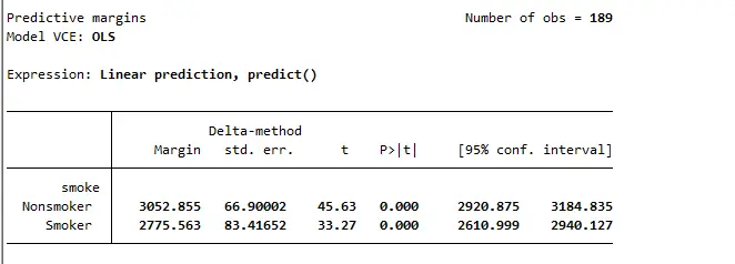
The above table shows that babies’ of non-smoker mothers are better off in terms of having more weight, compared to babies of smokers. As the saying goes, smoking is injurious to health. Well, that’s an information we have now verified from the data, too.
Now the individual effect has been explained, we now create the marginal plot that graphically represent the effect. We use the following command for creating marginal plot in Stata.
marginsplot
The following margins plot is generated in Stata
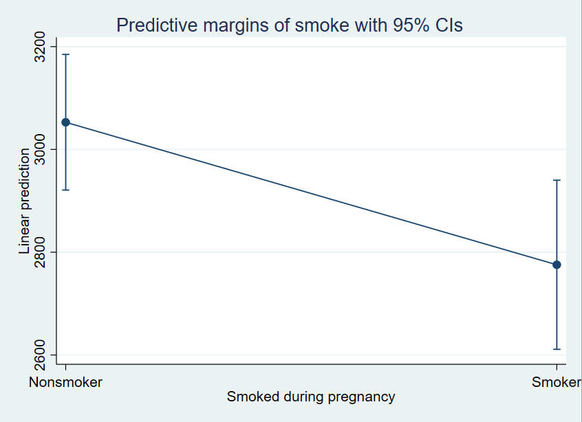
As the margin plot is just the visual representation of margins table, it also verifies the table that babies of non-smoker are weighed more than the babies of smoking mothers.
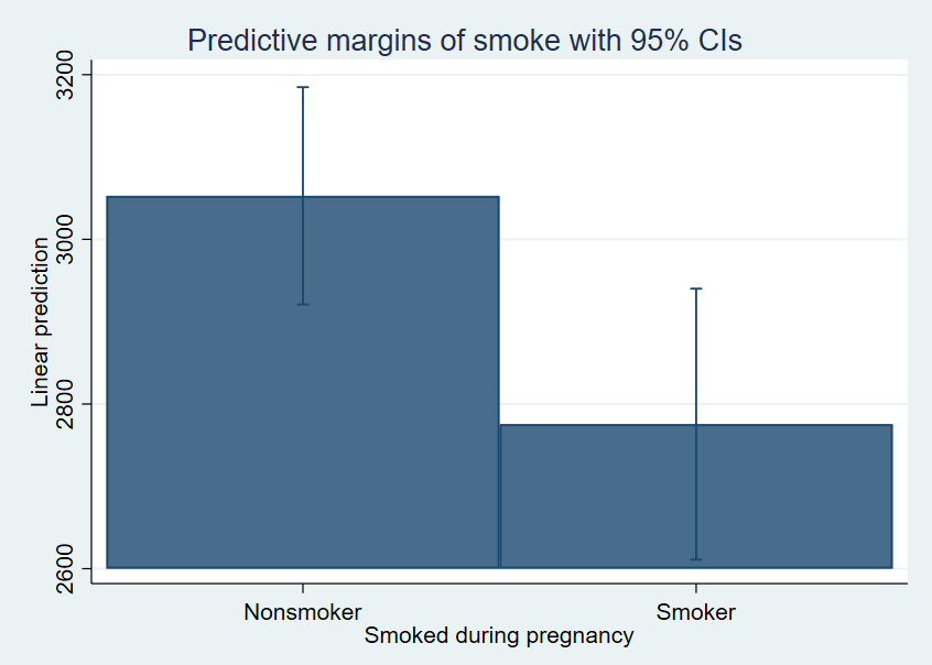
Although the graph shows the effect of smoking, it doesn’t visualize how much non-smoker mothers are better off with their babies’ health. To get this kind of visualization, we can get the bar graph by using the following command
marginsplot, recast(bar)
This command creates a type of bar chart as shown below. Now we can confirm that mothers who don’t smoke have babies with average weight of 3000 grams and are much better off, compared to smokers that have average weight of around 2700 grams.
Now that we have created graphs for the smoker and non-smoker categories, we can create margins for the respective ages of mothers too, and their effect on the birth weight of children. To create margins for the age of mothers, use the following command
margin, at(age= (18(3)30))
Let me walk you through this command first, in case you have a different data set with different values. The values (18(3)30) are the range of age, where 18 is the starting age and 30 is the ending age. The value 3 in parentheses is the increment of age by 3. So, in the above command we are taking age starting from 18 and incrementing it by 3 i.e. age 18, 21, 24 and so on , thus ending the age at 30.
The above command generates the following results in Stata
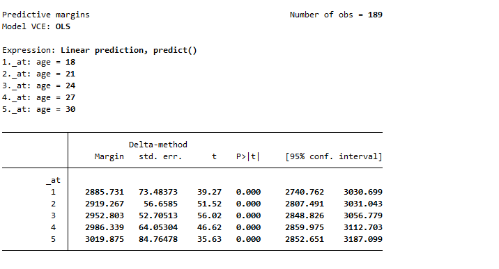
The birth weight of baby of mother aged 18 is around 2800 grams and the weight increases by the increase of age. To create a margin plot of the above table, we again use the following command that we used earlier
marginsplot
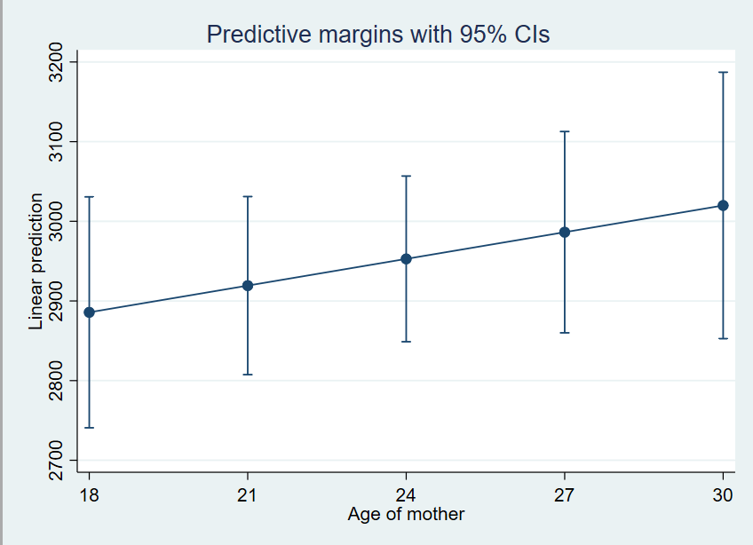
The margin plot again verifies the results table. However, the table and margin plot generated above doesn’t take into account the effect of smoking on the birth weight of babies, so to incorporate that effect, we use the following command
margin smoke, at(age= (18(3)30))
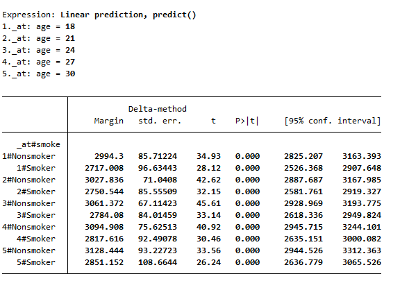
The above table generated explains the effect of age and smoking/nonsmoking combined on the birth weight in detail. Interpreting the above table, we can see that mothers at the age of 18 having smoking habits have babies with average weight of 2717 gram, compared to mothers with nonsmoking habits having babies with birth weight of 2994 grams.
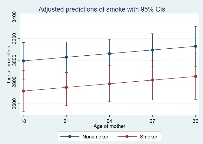
Similarly, the margins plot for this table will look like this, indicating that women with nonsmoking habits are clearly better off compared to their counterparts. To create a margins plot for the above table, use the following command
marginsplot
We can also create margins for the specific age too, whatever the requirement of data is. For instance, if we want to create a margin for the mother aged 35, we can use the following command
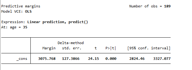
margin smoke, at(age=35)
The following margin table is generated, which describes that average weight of babies of mothers aged 35 is 3075 grams.
However, the above margin again doesn’t incorporate the smoking effect. To see the effect of smoking on weight of baby for mothers aged 35, we use the following command
margin smoke, at(age=35)
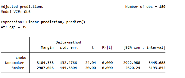
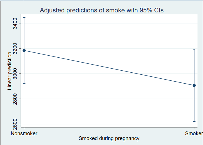
Now the margin table is generated that provides details about the weight of newborn babies, that changes depending on the smoking habits of their mothers. Again, the following margins plot is generated for the above margins., using the given command
marginsplot
Formatting of Margins Plots in Stata
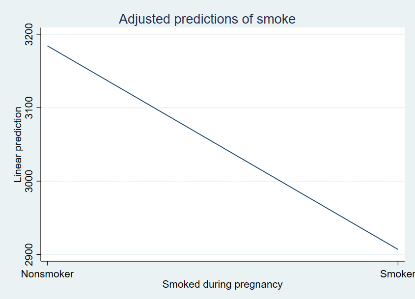
Now if we want to visualize this data graphically, one way is to simply create a margins plot, that will generate a graph similar to plots generated above. However, we can change that plot too, by incorporating a few features. If we want to create the margin plot by using the line plot and don’t add any confidence intervals into it, we can use the following command
marginsplot, recast(line) noci
The above command will generate following margins plot in Stata.
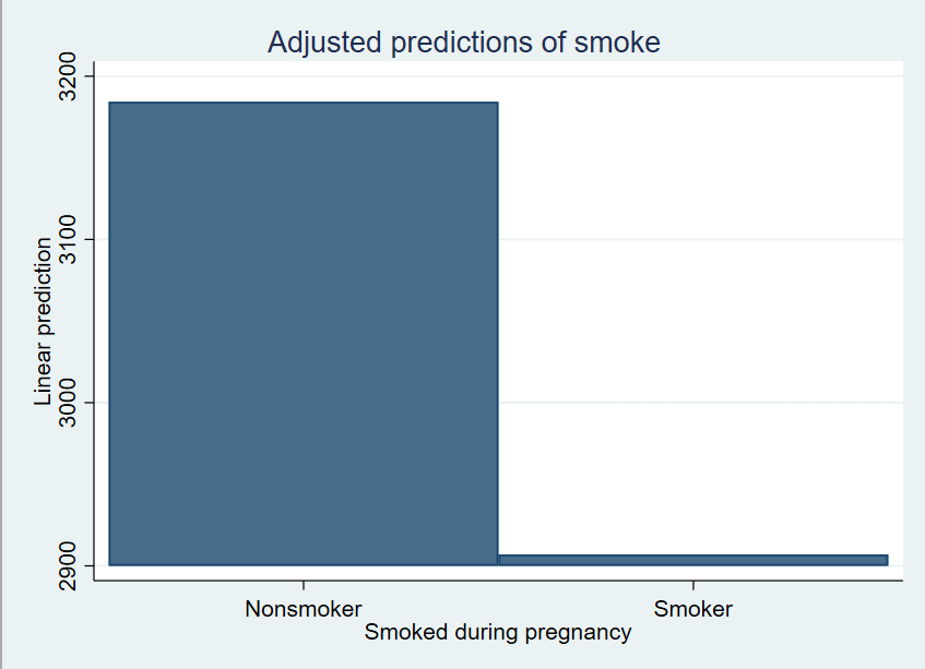
Similarly, if you want to have a better picture of data, the bar plot can be created in Stata. This bar plot can be generated using following graph, where y-axis is the marginal effects and x-axis is the categorical independent variable
marginsplot, recast(bar) noci
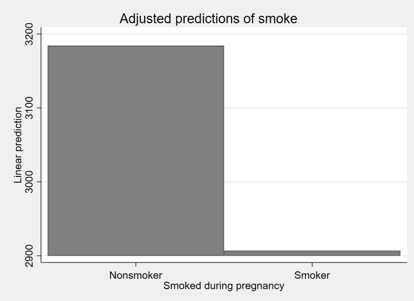
However, if you are a monochromatic person, where colorful graphs are not your thing, you can generate the monochrome graph using the following command.
marginsplot, recast(bar) noci scheme(s2mono)
The following monochromatic graph will be generated in Stata using the above command.
We can also give titles to our margins plot in Stata. To give a margin plot title, the following command will be used
marginsplot, recast(line) noci title("Difference of weights in babies of smokers and non-smoker mothers")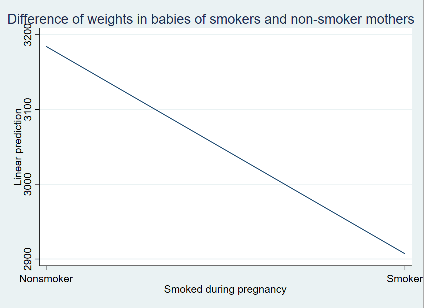
Only margins for the linear regression or linear model was covered in this article, however, the concept of margins is applied for the non-linear models too. Those nonlinear models whose marginal effects one wants to study include logit model, probit model or other non-linear models depending on your data.