
What are outliers?
Outliers are data points in a dataset that are different from the rest of the data. They can have immensely high or low values and can skew statistical analysis and models. Outliers can rise for various causes, including measurement errors, inaccurate data entry, or true abnormal events in the data. Finding and dealing with outliers is critical for data cleaning and robust analysis.
For deep understanding we will use the built-in dataset “mtcars”. Outliers in the mtcars dataset can be detect using a variety of methods, like z-scores, the IQR method, and visual inspection. Presenting some examples of how to utilize these approaches to find outliers in R using the dataset “mtcars”.
Using z-score
Z-score shows that how many standard deviations a data point is away. It is widely used approach in statistical analysis for accessing that whether our data contains outlier or not. Let’s understand it with an example.
#Load the dataset data(mtcars) # Calculate z-scores for the variable carb (Number of carburetors) in the dataset z_scores <- scale(mtcars$carb) # Identify outliers for carb variable based on a threshold (e.g., 3) outliers_z <- which(abs(z_scores) > 3, arr.ind = TRUE) # Print the row and column indices of outliers outliers_z
Outliers are discovered based on a defined z-score threshold (e.g., 3).
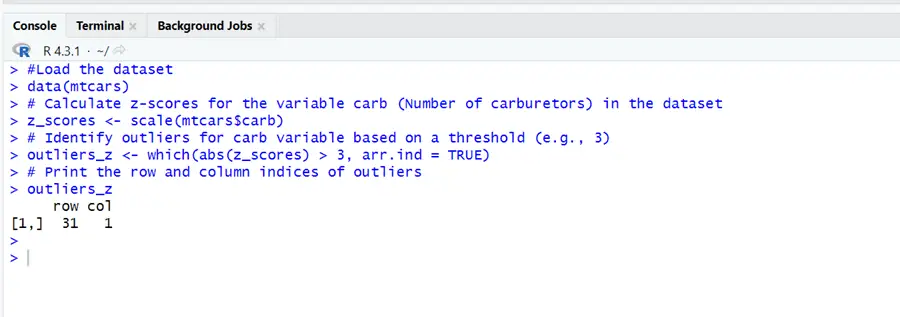
The method used above is Z-scores which identifies outliers in the “carb” variable of the ‘mtcars’ dataset, with a threshold of 3. The dataset mtcars contains an outlier in the “carb” variable. This anomaly can be seen at row index 31 and column index 1. This means that the number of carburetors (“carb” variable) for the car model at row 31 in the dataset has a Z-score greater than 3 standard deviations from the mean, making it an outlier in the context of this research. You may want to look into this data point more to understand why it differs from the rest of the data, or you may want to evaluate whether it should be treated differently in your analysis, based on your findings.
- IQR Method
In IQR method a range is defined by using first and third quartile and a multiplier which is usually set as 1.5. All the values below the lower limit and above the upper limit are consider as outliers. Have a look on the R code below.
# Load the mtcars dataset data(mtcars) # Define a multiplier for the IQR (e.g., 1.5) iqr_multiplier <- 1.5 # Create an empty vector to store outlier indices all_outliers_iqr <- c() # Calculate the lower and upper bounds for the carb variable lower_bound <- quantile(mtcars$carb, 0.25) - iqr_multiplier * IQR(mtcars$carb) upper_bound <- quantile(mtcars$carb, 0.75) + iqr_multiplier * IQR(mtcars$carb) # Find the indices of outliers outliers <- which(mtcars$carb < lower_bound | mtcars$carb > upper_bound) # Append the outlier indices to the all_outliers_iqr vector all_outliers_iqr <- c(all_outliers_iqr, outliers) # Get unique outlier indices all_outliers_iqr <- unique(all_outliers_iqr) # Print the row numbers of outliers all_outliers_iqr
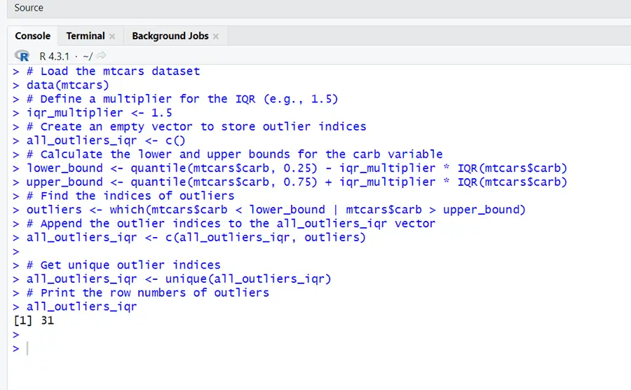
In this output all_outliers_iqr includes the row number of the data points considered as outliers using the IQR method with a multiplier 1.5. It represents that this row has a data point which exceeds the bound defined by IQR. Based on this strategy, row 31 in dataset contains an outlier. On depending the exact goals of investigation, one can further evaluate or process these rows.
- Box plot/Visual Inspection
Box plots are an effective technique for discovering and analyzing outliers in a set of data. Particular data points above the box plot’s whiskers are commonly used to represent outliers. Here’s how to make a box plot in R to find outliers. To visualize the outliers by boxplot we can use the boxplot function.
# Load the mtcars dataset data(mtcars) # Create a single boxplot with all variables displayed vertically boxplot(mtcars, outline = TRUE, horizontal = FALSE, col = "lightblue") # Outliers are the data points outside the whiskers of the boxplots
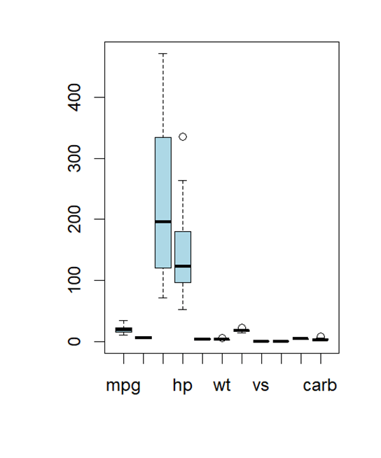
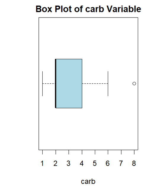
We can see the outliers in the above picture. For the separate boxplot you can use the code below:
# Load the mtcars dataset data(mtcars) # Create a box plot for the "carb" variable boxplot(mtcars$carb, main = "Box Plot of carb Variable", xlab = "carb", col = "lightblue", # Define the color of the box plot border = "black", # Define the color of the box outlines horizontal = TRUE # Display the plot horizontally )
One can connect all of these strategies and tailor the verge to find outliers based on individual analysis demands and desired level of sensitivity to outliers.
How to treat outliers in R?
Outliers can be treat in multiple ways in R. Below are some of these:
- Trimming
Trimming is the process of putting off a specific percentage of data points from both ends of a distribution. The trim function in R can be used for it.
By trim function:
# Install and load the robustbase package library(robustbase) # Load the mtcars dataset data(mtcars) # Set the proportion to trim from each end trim_proportion <- 0.1 # Sort the "carb" column sorted_carb <- sort(mtcars$carb) # Calculate the number of values to trim from each end n_to_trim <- round(length(sorted_carb) * trim_proportion) # Create the trimmed "carb" vector trimmed_carb <- sorted_carb[(n_to_trim + 1):(length(sorted_carb) - n_to_trim)] # Check the result summary(trimmed_carb)
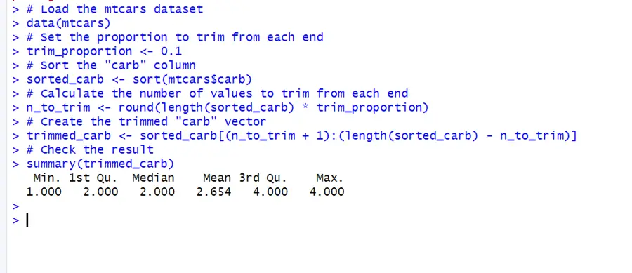
As you can see in the results trimming has worked effectively by cutting the 10 percent of values from both ends. Now the data is cleaned and free of outliers or extreme values.
- Transforming the data points
Transformations can be used to data to make it more frequently distributed. The log transformation, square root, and Box-Cox transformations are common examples of transformations. One of the example is given below:
# Load the mtcars dataset data(mtcars) # Apply the log transformation to the "mpg" column mtcars$carb_log <- log(mtcars$carb) # Check the result summary(mtcars$carb_log)
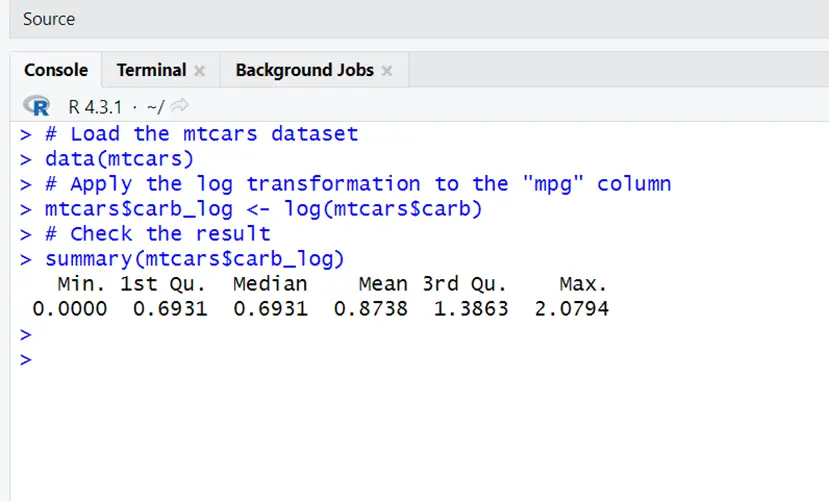
The data is logarithmically transformed and now used in the summary statistics for the “carb_log” column. When working with a wide range of values, this transformation can be useful for specific studies or visualizations when one wish to bring out the relative differences in the data on a logarithmic scale.
- Using the IQR Method:
The IQR is used to identify and deal with outliers. It is a measure of the spread of the data values. It is a reliable measure of dispersion because it is not affected by extreme values or outliers. To identify and remove outliers, the IQR is mostly used with box plots and other data visualization approaches. You can treat outliers by using the code below:
# Load the mtcars dataset data(mtcars) # Calculate the IQR for the "carb" variable carb_iqr <- IQR(mtcars$carb) # Calculate the lower and upper bounds lower_bound <- quantile(mtcars$carb, 0.25) - 1.5 * carb_iqr upper_bound <- quantile(mtcars$carb, 0.75) + 1.5 * carb_iqr # Define a multiplier value to replace outliers multiplier <- 2 # You can change this value to your desired multiplier # Replace outliers with the specified multiplier value mtcars_treated <- mtcars mtcars_treated[mtcars_treated$carb < lower_bound, "carb"] <- lower_bound * multiplier mtcars_treated[mtcars_treated$carb > upper_bound, "carb"] <- upper_bound * multiplier summary(mtcars_treated$carb)
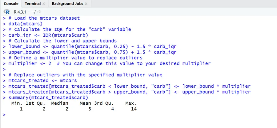
You can see that outliers have been removed from the mtcars dataset by interquartile range method. For this method you have to set a multiplier which helps to decide upper and lower limit.
- Using the Z-Score Method
A common technique for identifying outliers is to evaluate data points with a Z-score greater than a specific threshold (usually 2 or 3 standard deviations from the mean) as likely outliers. These data points differ highly from the normal and may be perceived uncommon. The code below is handling outliers by z-score method.
# Load the mtcars dataset if not already loaded data(mtcars) # Define a Z-score threshold (e.g., 3) z_score_threshold <- 3 # Calculate Z-scores for the "carb" variable z_scores <- scale(mtcars$carb) # Replace outliers with a fixed value (e.g., 3) mtcars_treated <- mtcars mtcars_treated[abs(z_scores) > z_score_threshold, "carb"] <- 3 # Summary of the cleaned carb summary(mtcars_treated$carb)
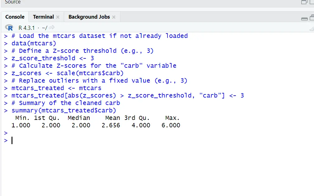
In the above result outlier has been removed by z-score method. This variable is cleaned now, which means it has no more extreme values. The code effectively removed the higher values from the carb variable.
- Using the Tukey’s Fences Method
The Tukey’s Fences method defines the bounds for detecting outliers using quartiles.
Data points that fall outside of the prescribed boundaries are called outliers and they can be identified, discarded, or handled appropriately. The code given below is representing the way of treating outliers by IQR in R:
# Load the mtcars dataset if not already loaded data(mtcars) # Define a multiplier for Tukey's Fences (e.g., 1.5) tukey_multiplier <- 1.5 # Calculate the IQR for the "carb" variable carb_iqr <- IQR(mtcars$carb) # Calculate the lower and upper inner fences inner_lower_fence <- quantile(mtcars$carb, 0.25) - tukey_multiplier * carb_iqr inner_upper_fence <- quantile(mtcars$carb, 0.75) + tukey_multiplier * carb_iqr # Calculate the lower and upper outer fences outer_lower_fence <- quantile(mtcars$carb, 0.25) - 3 * tukey_multiplier * carb_iqr outer_upper_fence <- quantile(mtcars$carb, 0.75) + 3 * tukey_multiplier * carb_iqr # Identify potential outliers (between inner and outer fences) potential_outliers <- which(mtcars$carb < outer_lower_fence | mtcars$carb > outer_upper_fence) # Replace potential outliers with NA mtcars_treated <- mtcars mtcars_treated[potential_outliers, "carb"] <- NA # Print a summary of the treated "carb" variable summary(mtcars_treated$carb)
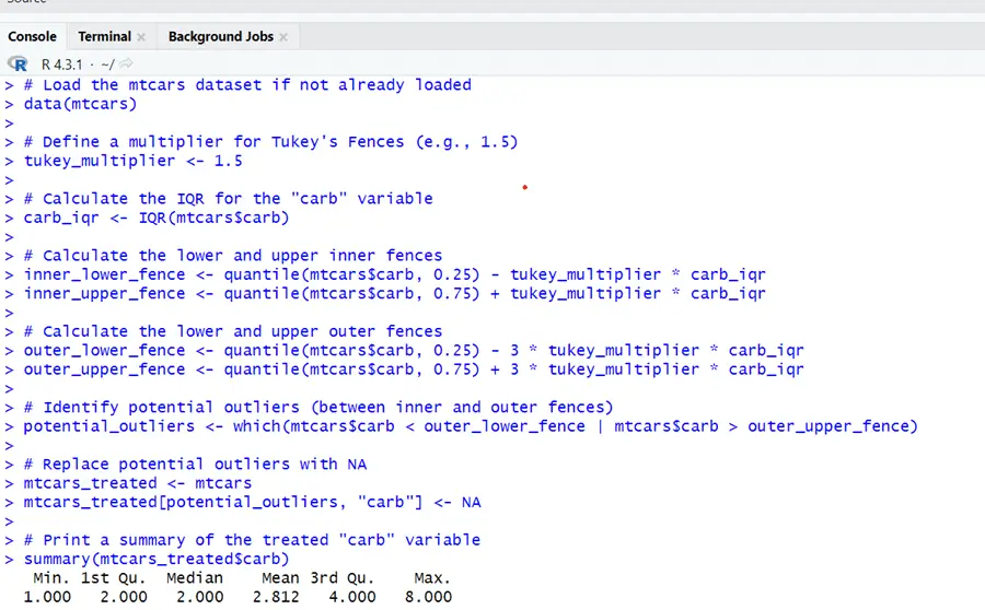
The results are showing the cleaned data without extreme values and outliers. Outliers have been removed from carb variable by Tuckey Fence Method.
- By Winsorization:
Winsorization is a data transformation technique that is used to minimize the impact of outliers in a dataset. It entails replacing outliers with less extreme data values, usually by limiting or trimming the extreme observations. The purpose of Winsorization is to reduce the sensitivity of the dataset to the impact of outliers. Here is the code for winsorization of carb variable from mtcars dataset. Below is the code for carb variable treated by winsorization.
# Load the mtcars dataset if not already loaded data(mtcars) # Set the lower and upper Winsorization percentages (e.g., 5%) lower_percentile <- 0.05 upper_percentile <- 0.95 # Calculate the lower and upper Winsorization values lower_value <- quantile(mtcars$carb, lower_percentile) upper_value <- quantile(mtcars$carb, upper_percentile) # Winsorize the "carb" variable by capping the extreme values mtcars_winsorized <- mtcars mtcars_winsorized$carb <- pmin(pmax(mtcars_winsorized$carb, lower_value), upper_value) # Print a summary of the Winsorized "carb" variable summary(mtcars_winsorized$carb)
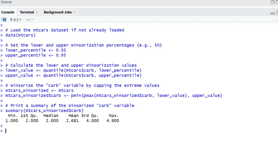
It can be seen from summary that outliers have been handled by this method by modifying extreme values in variable. Thus it reduces the impact of outliers in dataset by trimming them.
Each of these methods identifies and removes outliers from the `carb` variable by using different criteria. The resulting variables have outliers removed based on the respective criteria and method. One can choose the method that best fits their dataset and analysis.