
When working with linear regression models, it’s essential to assess the model’s assumptions and diagnostic tests. These diagnostics help us in ensuring the reliability of our regression analysis. In simple terms, they ensure that the results are correct and unbiased. In this tutorial, we will only focus on three crucial diagnostic tests: normality of residuals, heteroscedasticity, and multicollinearity. These three assumptions are integral to many regression models and are widely applicable.
Before we move to the diagnostic tests, make sure all the libraries are installed and loaded. Here’s how we can do it:
To install all the packages at once, just execute the following command:
install.packages (c("lmtest", "moments ","nortest", "car", "MASS", "multcomp", "tseries", "robust"))To Load the above libraries, execute:
library(lmtest) library(moments) library(nortest) library(car) library(MASS) library(multcomp) library(series) library(robust)
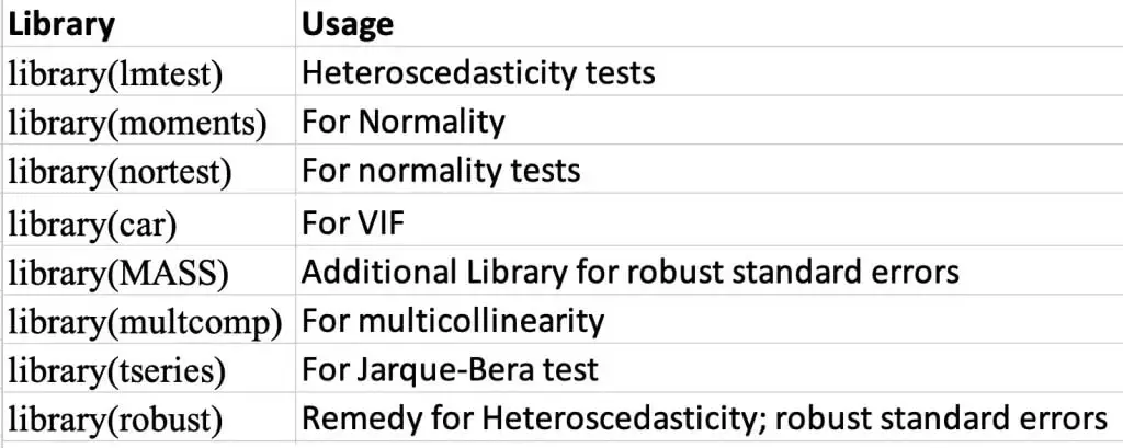
The following figure shows the use of these libraries:
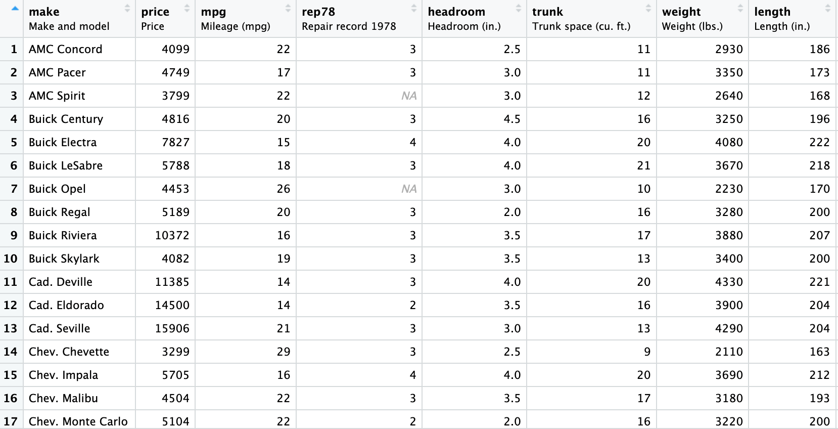
Again, we will be using the automobile data. Use the following commands to load and see the data:
auto <- read.csv("auto data.csv") View (auto)The Snapshot of the data is provided hereunder:
Now, let’s go through the three crucial diagnostic tests:
Normality of Residuals
The normality of residuals is one of the fundamental assumptions of linear regression. It states that the residuals (errors) should be normally distributed. In other words, means that the predictions made by the model are trustworthy. Let’s perform this test and analyse the results:
We start by performing the linear regression model using the following command:
model <- lm(price ~ mpg + weight + length, data = auto)
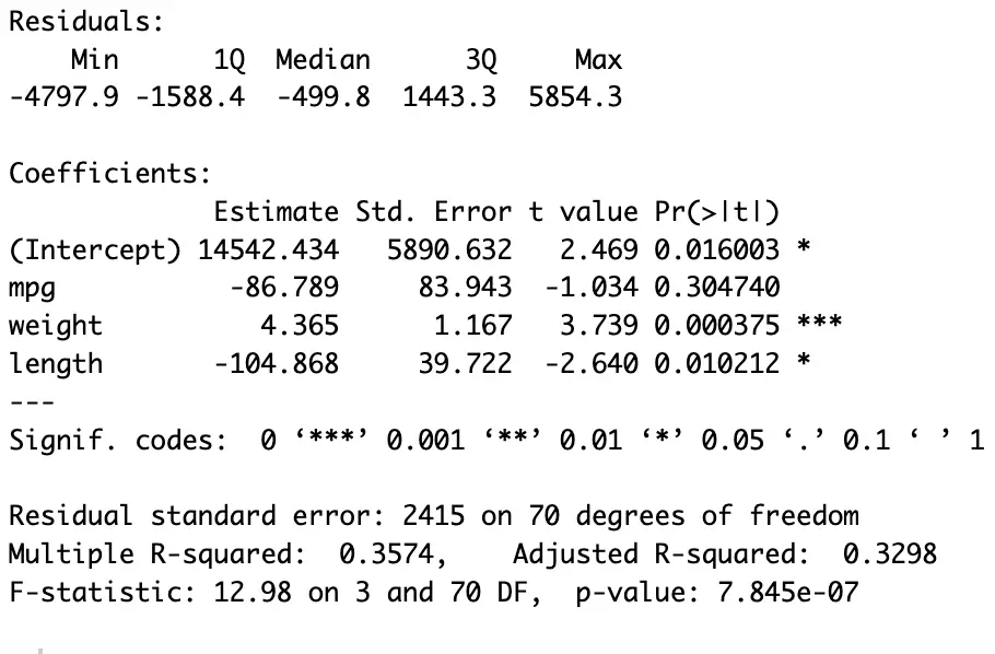
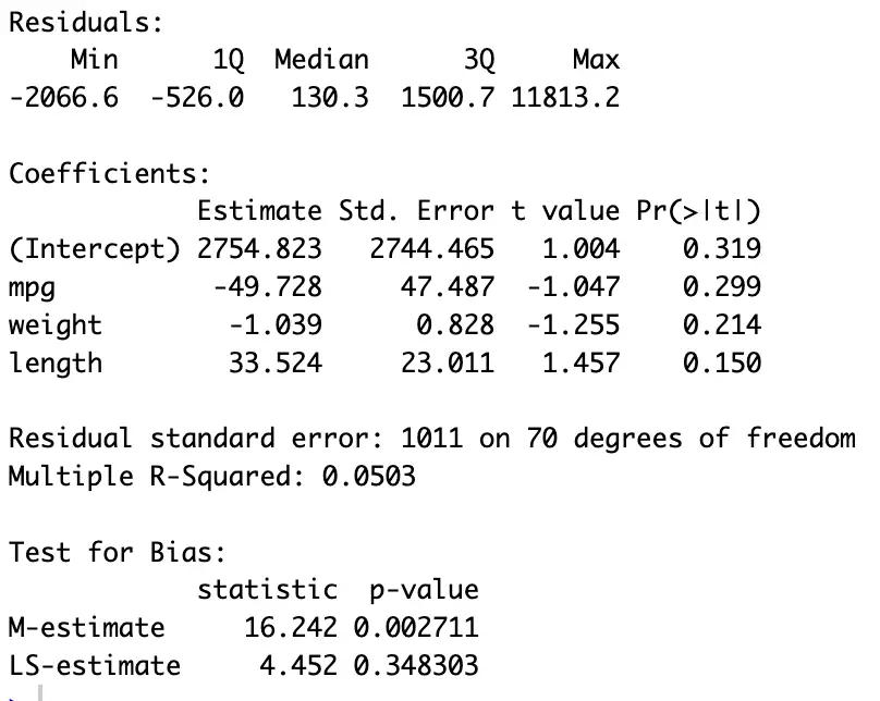
In the above command (see the last figure for the results), we have regressed [price] on [mpg], [weight], and [length] using the dataset named [auto]. The results are stored in [model].
For normality, we apply tests on the residuals. To Get the residuals (errors) execute:
residuals <- resid(model)
This command will store the residuals of the regression model in an object called [residuals]
Skewness, Variance, and Kurtosis
Skewness, Variance and Kurtosis tell us about the normality of data. Skewness tells us if our data is leaning to one side or the other, Variance shows how much our data points spread out, and Kurtosis helps us see if our data is unusually peaky or flat, and if there are any extreme values. Understanding these measures helps us make sense of our data’s behaviour and whether it’s normal or not. For instance, if data has mostly small values with a few really large ones, the average might not give the whole picture. If the skewness value is close to ‘0’ and kurtosis value is close to ‘3’, then the data is normally distributed.
To get skewness of the data, execute the following command:
skew <- skewness(residuals)
For Kurtosis execute:
kurt <- kurtosis(residuals)
For Variance execute:
variance <- var(residuals)
For the results use the following commands:
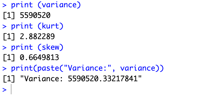
print (variance) print (kurt) print (skewness)
The print command displays the results stored in a variable. To display a specific name with the results use:
print(paste("Variance:", variance))This command will show the results with a given name in the command. Here we have given the name [Variance] to the result of variance. The results are here:
Normality tests
Nonetheless, we can use Normality tests, to confirm that our data is normally distributed. They provide additional information about our data by quantifying the degree of normality; and how closely our data aligns with the normal distribution.
For normality, we can use the following two tests:
Shapiro-Wilk test
To perform the Shapiro-Wilk test execute the following command:
swilk <- shapiro.test(residuals)
For Jarque-Bera test use:
jb_test <- jarque.bera.test(residuals)
For the results execute the following command
print(swilk) print(jb_test)
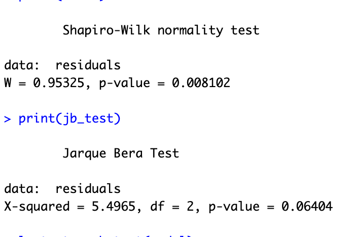
The null hypothesis in these two tests is, that the data is normally distributed. However, a p-value less than 0.05 suggests that the residuals are not normally distributed, or in other words, it rejects the null hypothesis. In such cases, we should transform our data or apply non-linear regression models if the normality assumption is violated.
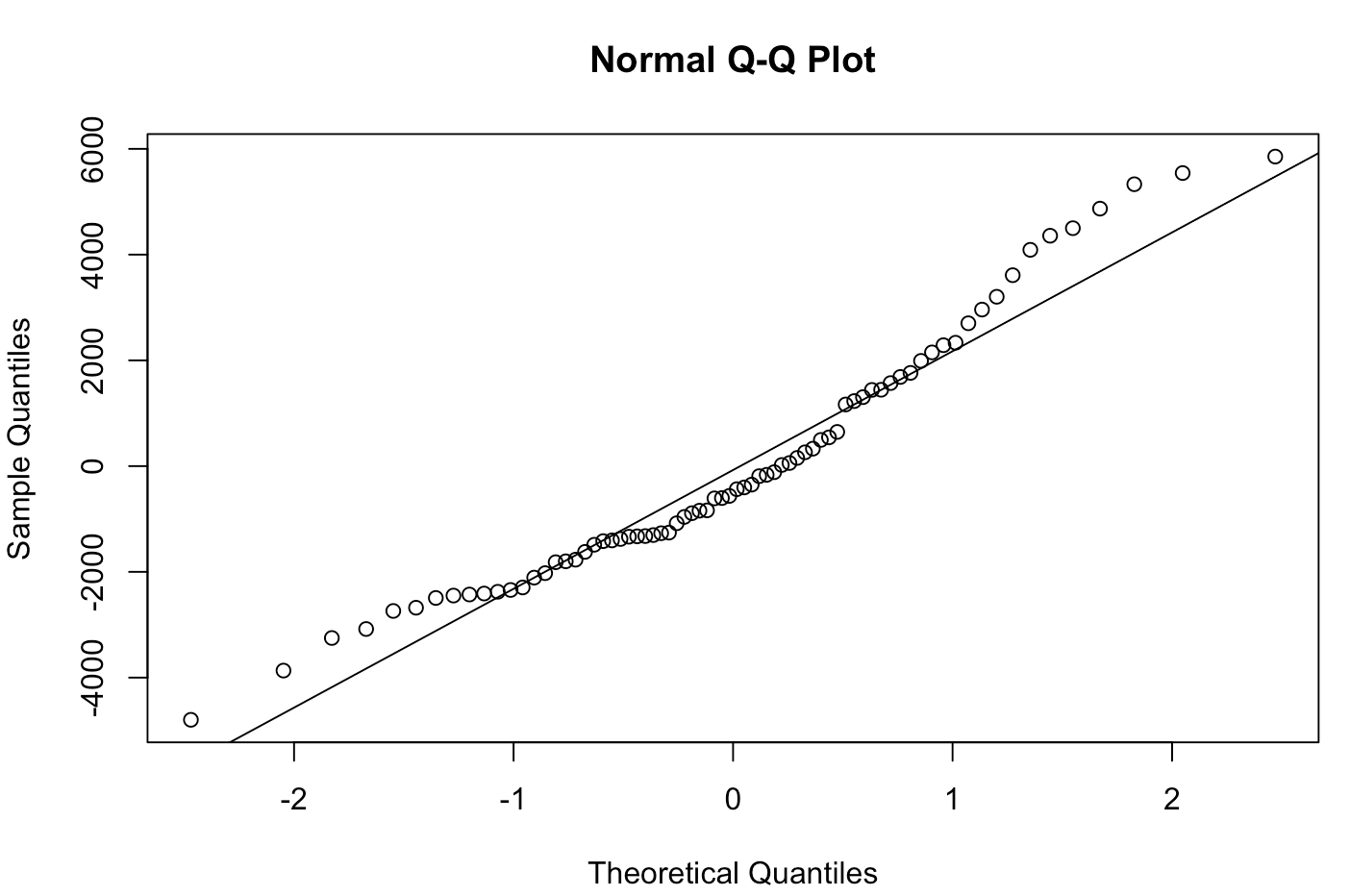
QQ Plots for Residuals
Another way of looking at normality is using QQ (Quantile-Quantile) plots. QQ plots are a useful graphical tool to assess the normality assumption of residuals. They compare the quantiles of the residuals to the quantiles of a theoretical normal distribution, which is a benchmark for data. If the residuals are normally distributed, the points on the QQ plot should form a roughly straight line. Here, the distance from the straight line shows departures from normality. It is a precise way to visually assess whether the residuals follow a normal distribution.
To create a QQ plot for your residuals and add a reference line to it, we can use the following commands:
qqnorm(residuals) qqline(residuals)
The `qqnorm` function creates the QQ plot, and the `qqline` function adds a reference or benchmark line.
The results of the QQ plot are here:
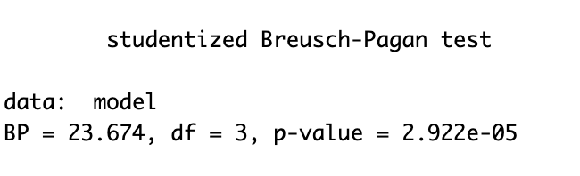
Heteroscedasticity
Heteroscedasticity refers to the unequal spread or variance of residuals. This means that the data points are not equally spread out; some data points are spread far apart. To detect heteroscedasticity, we can use the Breusch-Pagan test and the LM (Lagrange Multiplier) test. Here’s how we can perform these tests:
Breusch-Pagan test
For the Breusch-Pagan test execute:
het_test <- bptest(model)
To see the results execute
print(het_test)
Lagrange Multiplier test
Similarly, for the LM test use the following command:
lm_test <- bgtest(model) print(lm_test)
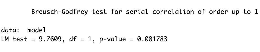
If the p-value from these tests is less than 0.05, it indicates the presence of heteroscedasticity. We need to search for a remedy to address this issue. The results of both tests are presented in the above figures. Note: The results of a test depend on its underlying formula and the sample size. Two different tests of normality can give different results.
One remedy often used is the robust regression model. Which creates corrected unbiassed error terms which are distributed normally. To perform robust linear regression model, execute:
robust_lm_model <- lmRob(price ~ mpg + weight + length, data = auto)
To see the summary of the robust regression model use:
summary(robust_lm_model)
the results of the robust (corrected) regression model are hereunder:
Multicollinearity
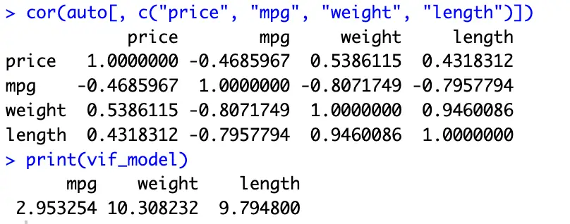
Multicollinearity occurs when two or more predictor variables in your model are highly correlated. It can lead to incorrect and unstable coefficient estimates. In such cases, there are variables which don’t give us extra information but are incorporated in the model. We are to differentiate which variable is more important for the model. In our case, we may be unable to differentiate between whether the price is increased due to the weight or length if these two variables are correlated. We can check for multicollinearity using the Correlation Matrix and Variance Inflation Factor (VIF).
Calculate the correlation matrix
cor(auto[, c("price", "mpg", "weight", "length")])The above command will show the correlation matrix for the above four variables. A value close to zero suggests multicollinearity.
However, we can also confirm it via Variance Inflation Factor (VIF)
Calculate the Variance Inflation Factor (VIF) for the model
VIF quantifies the degree of multicollinearity between predictors in our model, helping in identifying the variables which are highly interrelated and might need adjustment.
To calculate the VIF values use the following command:
vif_model <- vif(model)
To see the results of VIF test execute the following command.
print(vif_model)
If any VIF value is greater than 10, it suggests high multicollinearity, and we should consider removing one of the correlated variable from our model. The results of VIF and the correlation matrix are provided here:
In summary, diagnosing your linear regression model is a crucial step in regression analysis. These three diagnostic tests for normality of residuals, heteroscedasticity, and multicollinearity help ensure the reliability of our model and guide us in making necessary adjustments. Addressing these issues can lead to more accurate and robust regression results. For more diagnostics and assumptions tune into thedatahall.com