
In econometric models, some variables can play a very important role in the explanation of an economic phenomenon. For instance, gender can play a crucial role in determining salary levels. However, quantifying gender isn’t straightforward because gender lacks a numerical nature. This tutorial aims to explain methods for incorporating such information into econometric models, employing ‘dummy’ variables, using R.
We begin our analysis by installing and loading the necessary libraries. To accomplish this task, execute the following commands:
install.packages (c("ggeffects", "ggplot2")) library(ggeffects) library(ggplot2)To load the data, simply execute the following command:
set.seed(123) data <- data.frame( id = 10001:10500, age = sample(20:45, 500, replace = TRUE), marks = sample(20:100, 500, replace = TRUE), salary = sample(1000:5000, 500, replace = TRUE), gender = sample(c('Male', 'Female'), 500, replace = TRUE), education = sample(c('Primary', 'Secondary', 'Bachelor', 'Masters'), 500, replace = TRUE))The [set.seed(123)] command ensures that running the code again will yield the same random sample as the initial run. The second command creates a hypothetical dataset which is required for the regression analysis, utilizing the symbol [<-] to store the results or values in a new variable.
Note: Our dataset is a randomly generated sample made for this analysis, and it may not precisely portray real-world scenarios.
To see a snapshot of our data, use the following command:
View(data)
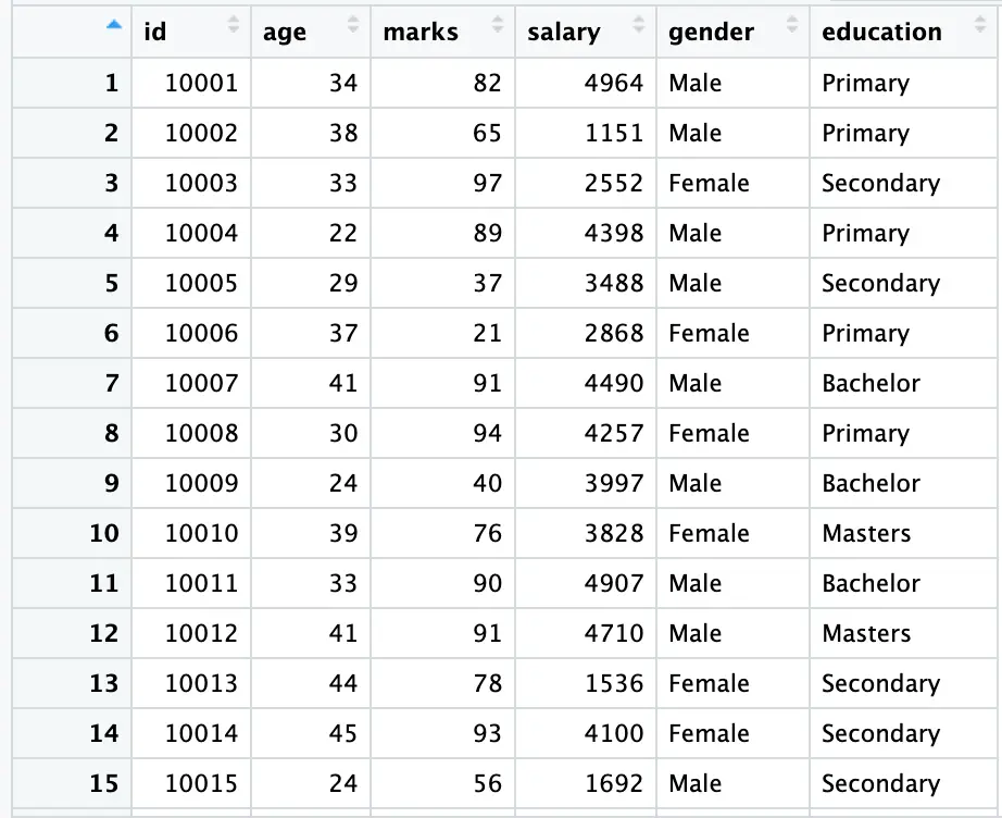
In the above figure, the gender variable is a string variable; a variable without numerical values. To address this, we will assign codes (1 and 0) to ‘Male’ and ‘Female,’ creating two new variables in our data using the following commands:
data$male <- ifelse(data$gender == 'Male', 1, 0) data$female <- ifelse(data$gender == 'Female', 1, 0)
The [ifelse()] function is employed here to generate two dummy variables, ‘male’ and ‘female,’ utilizing [$] to extract gender information from our [gender] column. In the [male] column, it assigns the value 1 when the gender is [Male] and 0 when it is [Female]. The same logic is applied to the ‘female’ column, with opposite values assigned to each gender; ‘female’ receives 1, and ‘male’ receives 0.
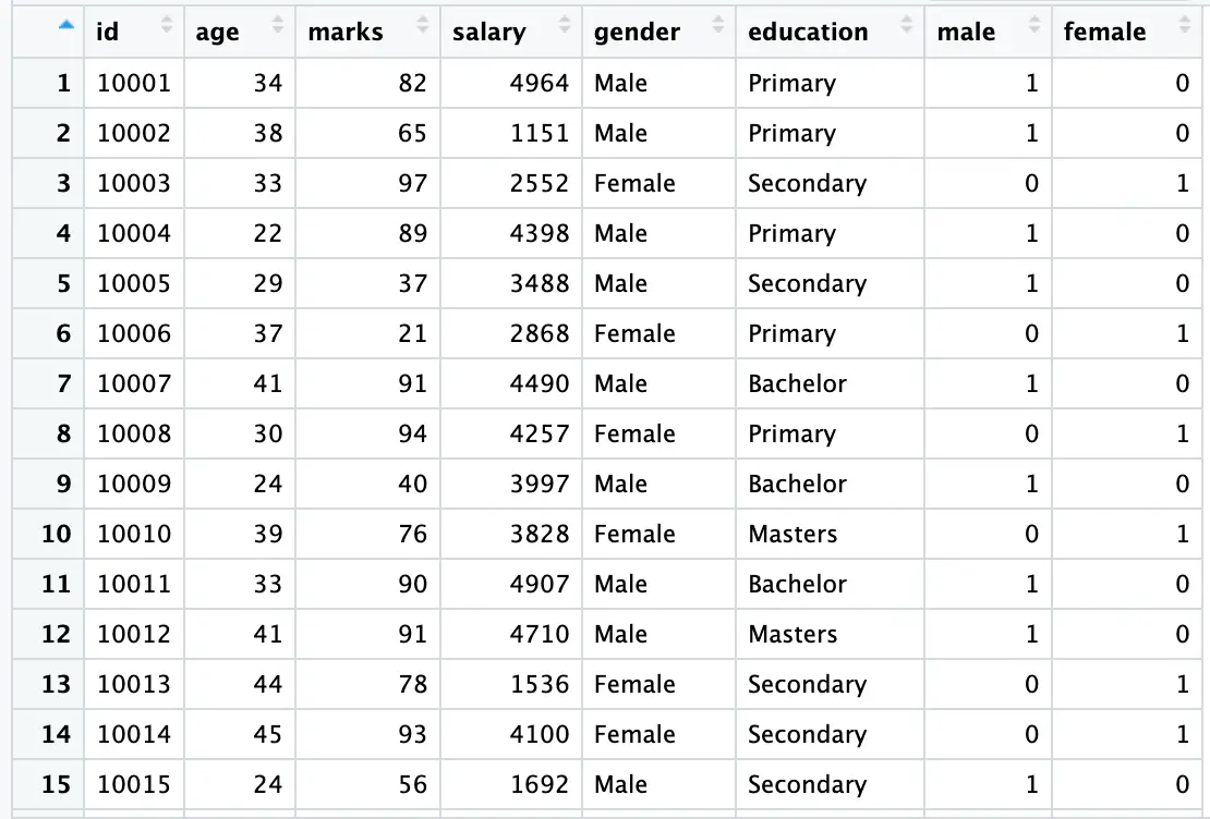
To review the updated data, execute the following command again:
View(data)
This will display the dataset, with the newly created [male] and [female] variables.
Dummy Regression (Manual Approach)
Having manually generated data for dummy regression, we now have both male and female dummy variables. To conduct dummy regression for both male and female, execute the following commands:
model_male <- lm(salary ~ male, data = data) model_female <- lm(salary ~ female, data = data)
The [lm] function is used to fit a linear regression model, regressing salary as a function of being male or female. This command avoids the dummy variable trap by omitting one category, which helps prevent multicollinearity issues and ensures the model’s stability and interoperability. (More details about multicollinearity are provided here)
To examine the results of the male regression model, use the following command:
summary(model_male)
The [summary] command provides an overview of the regression model, presenting coefficients, p-values, and other statistics. The output of the male regression model (male is taken as the benchmark category) is displayed in the figure below using the [summary] command:
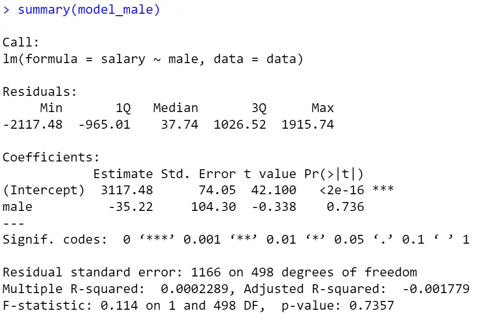
In our model, as depicted in the figure above, the results indicate that, on average, a male will earn $35 less than a female (the negative sign shows a decrease in salary).
To view the model’s result with [female] as the benchmark dummy, execute the following command:
summary(model_female)
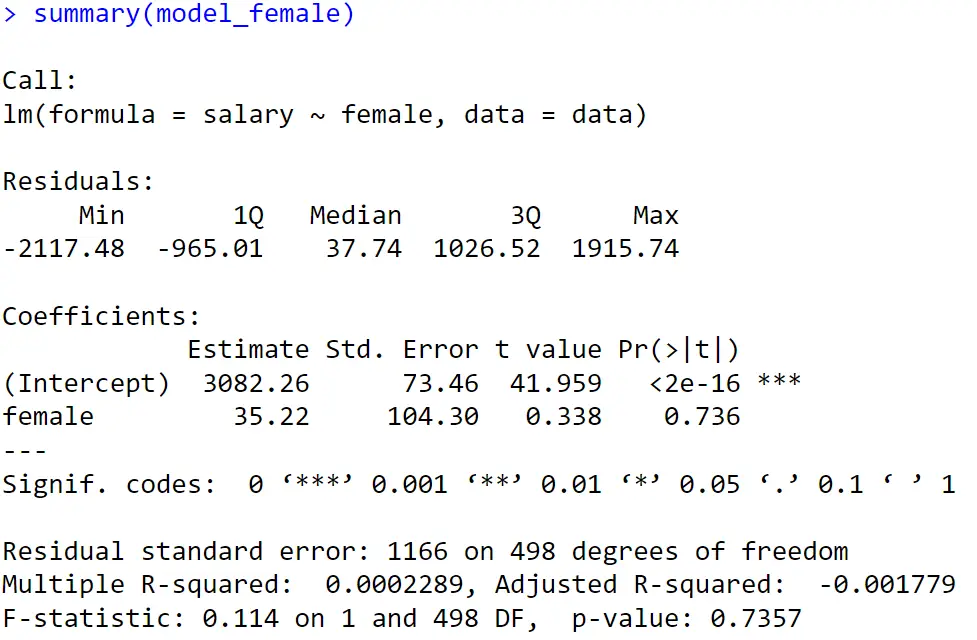
For the regression model concerning females, the intuition behind is the same, the results indicate that, on average, females will earn $35 more than males (see the above figure).
Note: In dummy regression, the intercept term depicts the omitted category, so the intercept term of one model must be equal to the results of the second model. We can confirm this by performing the following exercise:
result <- 3082.26 + 35.22 print(result)
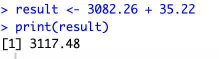
Here [3117.48] is the intercept of the first model. This is calculated by adding the intercept and slope of the second model(female).
Regression Analysis (Built-in Approach)
A more convenient way to do the dummy regression is the built-in approach. The results of both regressions are the same. However, the built-in approach helps in more complex dummy regressions; when we have more than one dummy. Moreover, it also helps in the graphical analysis of dummy regression.
In this approach, we code our gender variable using the following command:
data$gender <- factor(data$gender)
the above command gives numerical values to our gender variable using information stored in [data].
After generating the required dummies, we again regress salary on gender.
builtinmodel <- lm(salary ~ gender, data = data)
This command Converts ‘gender’ to a factor and runs a regression model with ‘gender’ as a predictor for ‘salary’.
For the results execute the following command.
summary(builtinmodel)
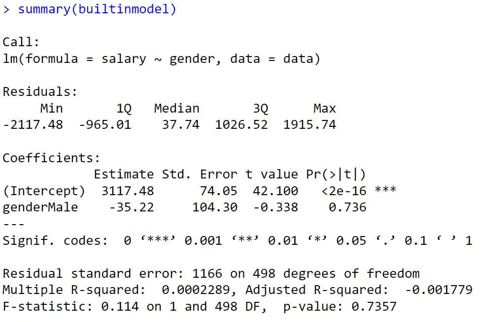
From the beginning of this tutorial, we have two dummies; male and female. Sometimes we don’t know which dummy is taken by our model as the benchmark and which one is omitted. In such cases just execute the following command:
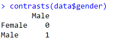
contrasts(data$gender)
This command will assign the value [1] to the benchmark category and [0] to the omitted category.
The results of our last command are presented in the following figure:
Marginal Effects Plot
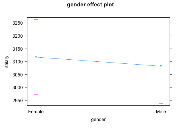
Marginal Effects Plots provide a visual representation of the impact of an independent variable on a dependent variable in regression analysis. In the context of dummy variable regression, such as the regression of salary on gender, Marginal Effects Plots are particularly useful. These plots showcase the change in the predicted value of the dependent variable (salary, in this case) when transitioning from one category of the dummy variable (e.g., male) to another category (e.g., female).
To create a Marginal Effects Plot for the regression of salary on gender, we can utilize the following commands:
model_plot <- lm(salary ~ gender, data = data) marginal_effects <- ggpredict(model_plot, terms = c("gender")) plot(marginal_effects)This sequence of commands fits a linear regression model [lm()] for salary regressed on gender. The [allEffects()] function is then used to calculate the marginal effects for both [male] and [female]. Finally, the [plot()] function is employed to display the Marginal Effects Plot in the output window. This graphical representation can provide a clearer understanding of the relationship between salary and gender in our regression analysis. The pink line shows the confidence interval. A confidence interval is a range showing where the true value is likely to be.
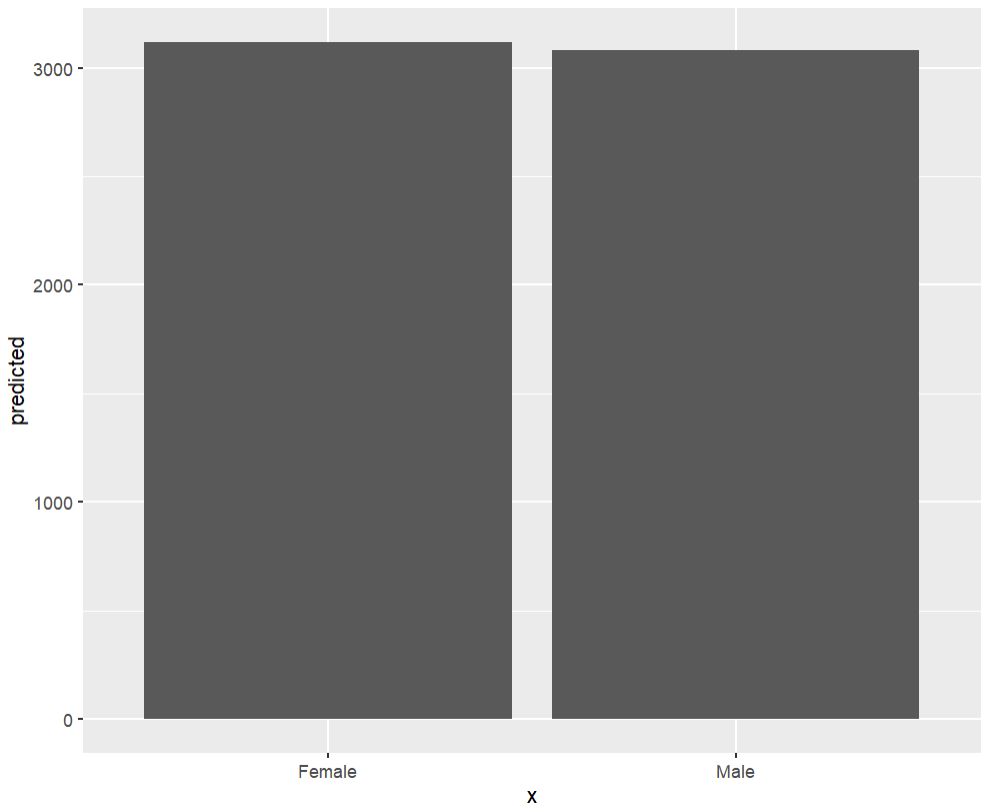
When comparing two categories (as in our case), bar plots are often considered more convenient. Execute the following commands for the barplot visualization:
ggplot(marginal_effects, aes(x = x , y = predicted)) + geom_col()
The above code uses ggplot function from ggplot2 package. Using the same marginal_effects object we created, I have provided the x and y axis variables into ggplot function.
To learn more on how to make graphs related to categorical variables in ggplot click here.
This tutorial serves as a starting point in dummy regression analysis. However, in dummy regression, we often encounter more than one category. To learn how to incorporate such information into our econometric analysis and present it graphically, stay tuned to thedatahall.com.