
ANCOVA is a statistical term that is used to compare the means of a dependent variable among two or more groups and co-variates. It combines the ANOVA and regression as it contains at least one categorical (factors) and one continuous (covariates) independent variable. Co-variates, known as confounding variables, are continuous independent variables in the model that are not of our main interest. ANCOVA is used to test whether the population mean of an outcome variable is the same across levels of independent categorical variables while controlling the effect of co-variates (continuous variables). It helps us to increase the precision of estimates and lessen the likelihood of type-I error by accounting for the source of variability in the data.
Assumptions of ANCOVA
ANCOVA has some similar assumptions to ANOVA and regression, like normality, independence, and homogeneity, although it has more assumptions to meet to ensure the validity and reliability of the model.
Linearity, which asks for the linear relationship among covariates and dependent variables,. It means that the change in the dependent variable is constant for one unit change in the covariate. To check this assumption, one can use the ggplot() function in order to find the linearity of variables.
The assumption of homogeneity of variance also has to be met. The variance of the dependent variable should be equal across various levels of factors. Levene’s test can be used to check this assumption of homogeneity of variances.
The normality of residuals is one of the assumptions of ANCOVA. It is essential to check the normality of residuals. The Shapiro-Wilk test can be used to check the normality of residuals.
We can also check more assumptions like homogeneity of regression, multicollinearity, etc.
One-Way ANCOVA
One-way ANCOVA contains a categorical variable and one co-variate, as it is an extension of one-way ANOVA. Co-variates included in the variable are linearly related to the dependent variable. The inclusion of co-variates increases the accuracy of detecting differences between various groups of independent variables. A typical one-way ANCOVA model looks like this:
Yij= β0+ β1Xij + β2Zi+ 𝓔ij
Where Yij is the dependent variable, β0, β1,β2 are parameters, and Xij is the independent variable. Zi is the covariate of the ith group, and 𝓔ij is the error term. It compares the means across different levels of factors while controlling the effect of co-variates in order to test whether there are statistically significant differences in means across groups.
The hypothesis that will be used for this questions is that
Ho: There is no significant difference in mpg across different gear types while controlling the weight of the car.
H1: There is significant difference in mpg across different gear types while controlling the weight of the car.
Below is the code for one-way ANCOVA.
Let’s understand these with an example from the built-in dataset of mtcars. We will use two variables: car weight (wt) and miles per gallon (mpg). The hypothesis we are going to check is that while controlling the effect of car weight, does the number of gears (3, 4, and 5) have a significant impact on the miles per gallon (mpg) of the car?
Below is the code for one-way ANOCOVA.
# Load necessary libraries library(ggplot2) library(car) # Load the mtcars dataset data(mtcars) # Assumptions Check # Checking linearity ggplot(mtcars, aes(x = wt, y = mpg, color = as.factor(gear))) + geom_point() + geom_smooth(method = "lm", se = FALSE) + labs(title = "Linearity Check") # Check homogeneity of variances leveneTest(mpg ~ as.factor(gear), data = mtcars) # Check normality of residuals shapiro.test(model$residuals)
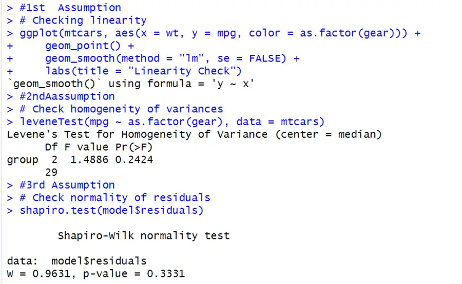
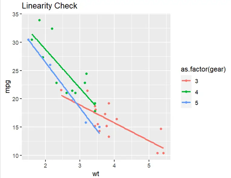
The above plot shows a linear relationship among these variables and co-variates. Hence, it fulfills the assumption of linearity. Homogeneity test results are insignificant as the p-value is greater than 0.05. It shows that variances do not have a significant effect across levels of gears. So, this assumption is fulfilled too. The normality assumption is also fulfilled as the p-value is larger than 0.05. This shows that residuals are normally distributed. Now we can perform ANCOVA as all our assumptions are fulfilled.
# Conduct ANCOVA ancova_model <- lm(mpg ~ wt + as.factor(gear), data = mtcars) summary(ancova_model)
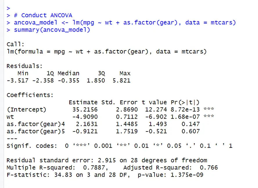
It can be seen in the results that wt has a highly significant effect on mpg. One unit increase in car weight will result in a 4.9-fold decrease in miles per gallon. The reference category is 3 by default. R-squared value shows that 79% of the variation is explained by the model. Gears do not significantly contribute to mpg while controlling the effect of the wt variable.
Two-way ANCOVA
A two-way ANCOVA contains two categorical variables (independent) and one continuous (co-variate). It is an extension of one-way ANCOVA, which examines the main effects and interaction effects between two factors while controlling the effects of covariates. Its model looks like this:
Yijk= β0+ β1Xij+ β2Zi + β3Wk + β4(XZ)ij+ 𝓔ijk
Where, Yijk is the dependent variable of the kth observation in th jth level of the second factor in the ith level of first factor. Xij and Wk are first and second factors simultaneously. Zi is the co-variate of ith group. (XZ)ij is the interaction term. It tests that whether there is any significant main and interaction effects between two factors on outcome variable while controlling the effect of co-variates. Hypothesis for two way ANOCOVA is that at least one mean dependent variable vary across the independent variables with some interaction.
Ho: At least one of the means of mpg vary across the level of categorical variable gear and cyl.
H1: All the means are same for mg across different levels of gear and cyl.
Below is the code for two-way ANCOVA.
# Load necessary libraries library(ggplot2) library(car) # Load the mtcars dataset data(mtcars) # Assumption Checks # Homogeneity of Variances leveneTest(mpg ~ as.factor(gear) * as.factor(cyl), data = mtcars) # Normality of Residuals ancova_model <- lm(mpg ~ wt + as.factor(gear) * as.factor(cyl), data = mtcars) shapiro.test(ancova_model$residuals)
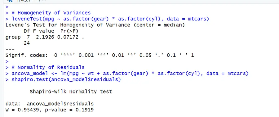
Assumption of linearity for ANOCOVA is same as the above in one-way ANOCOVA. In homogeneity test p-values are larger than the typical significant level which move us to the acceptance of null hypothesis that there is no difference in the variances. Normality assumptions is also fulfilling as p- value here is also greater than 0.05. So we can move further for the interpretation of two-way ANOCOVA.
# Conduct Two-Way ANCOVA ancova_model <- lm(mpg ~ wt + as.factor(gear) * as.factor(cyl), data = mtcars) summary(ancova_model)
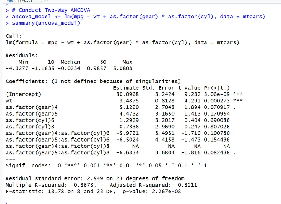
Percentage of variation explained by independent variables (gear, cyl, wt) in dependent variable (mpg) is 82.11. All the variables except wt have insignificant impact in model. The impact of gear variable on mpg depend on its specific levels. Cars with 4 gears has estimated increase of 5.1220 in the average mpg compared to the reference category 3.
Hence, ANOCOVA is a valuable tool in experimental design in order to check the influence of continuous variable while comparing the groups.