
Introduction
Many econometric models often get afflicted by what is called the endogeneity problem. This happens when one or more independent variables are correlated with the error term (omitted variable bias), or when the dependent and independent variables jointly determine each other (simultaneity bias).
This problem needs to be addressed because in the presence of endogeneity, OLS regression results end up being inconsistent and biased, and we cannot make any causal inferences between our variables of interest. This is because endogeneity means that our dependent and independent variables move together only because a change in the independent variable leads to a change in the error term, which in turn moves the dependent variable.
One of the ways this problem of endogeneity can be addressed is through the use of instrumental variables using the Two-Stage Least Squares (2SLS) approach.
One of the most well-known examples of endogeneity caused due to simultaneity bias is the demand function in microeconomics where price and quantity demanded are jointly determined. Omitted variable bias can be seen in examples like the regression of wage on education since a person’s earnings are not just a function of their education but also a host of other factors that are present in the error term.
So, what are instrumental variables and how are they used in the Two-Stage Least Squares (2SLS) approach to fix the endogeneity problem?
Instrumental Variables (IVs)
Before getting into how a two-stage least square regression analysis is done, let’s get a quick idea about what instrumentals are. They are, after all, ‘instrumental’ to the analysis!
Remember that endogeneity arises when an independent variable is correlated with the error term which is a violation of one of the key assumptions of a classical regression model.
Instrumental variables (IVs) are variables that are not correlated with the error term but are correlated with the independent variable [Corr(Z, e) = 0 and Corr(Z,x) != 0]. Secondly, they must affect the dependent variable only through the independent variable, i.e. a valid IV should not have a direct effect on the dependent variable of interest.
By using a variable with these characteristics, a causal relationship between the dependent and (endogenous) independent variable can be estimated with the endogeneity bias or inconsistency affecting the results.
What is Two-Stage Least Squares (2SLS)?
Two-Stage Least Squares (2SLS) is a two-step regression method that makes use of instrumental variables to address issues like endogeneity bias.
In theory, two regressions are run.
The first-stage regression regresses the endogenous independent variable on the instrumental variable and all the exogenous variables in the model. This helps us obtain the predicted values for the endogenous independent variable (x_hat). In case of a good and valid IV, the first-stage regression will have a statistically significant parameter.
In the second-stage regression, the dependent variable in our original model is regressed on x_hat, and the rest of the exogenous variables.
The parameter for x_hat from the second-stage is devoid of endogeneity bias and gives us bias-free, consistent estimates.
2SLS Regression in Stata
In this article, we will make use of the WAGE2.dta dataset that can be downloaded from here.
We can run a 2SLS regression in two ways: running the first-stage, obtaining x_hat, and using it to run the second stage. Or use the ivregress 2sls command to run the entire model. We will start with running both regressions one by one.
use WAGE2.dta
We are interested in seeing the effect of one’s education on their wages. We would also like to add controls for a person’s work experience, marital status, race and area of residence. Our model would look something like this:
wage = B0 + B1educ +B2exper + B3married + B4black + B5urban + error
This is also called the structural equation.
However, education (‘educ’) is an endogenous variable that is correlated with many variables in the error term – such as one’s own inherent abilities. Therefore, we cannot estimate the structural equation via a typical OLS regression.
We can address this endogeneity by using a person’s IQ score as an instrumental variable for ability. It satisfies the assumptions of a valid IV in that it is correlated with one’s education, but does not directly affect one’s wages. IQ will only have an effect on wages through education.
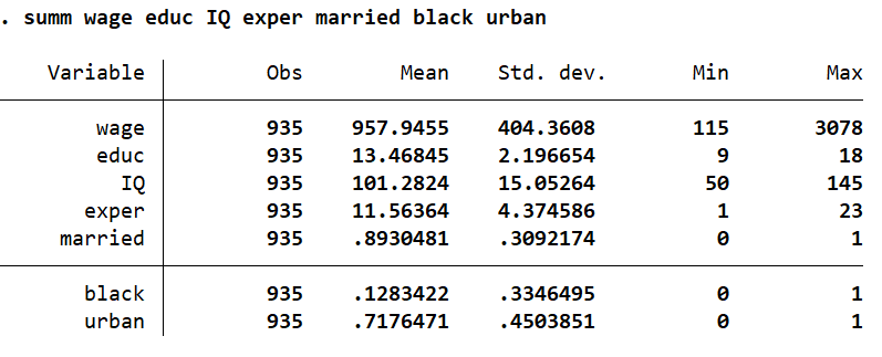
Let’s summarise all of the variables we will be using.
summ wage educ IQ exper married black urban
First Stage of 2SLS in Stata
As mentioned, the first stage of a 2SLS model is the regression of our endogenous independent variable (‘educ’ ) on the instrumental variable (‘IQ’) and other exogenous variables (‘exper’, ‘married’, ‘black’, ‘urban’) in the model.
educ = a0 + a1IQ +a2exper + a3married + a4black + a5urban + error
reg educ IQ exper married black urban
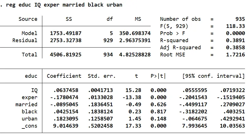
We will now obtain the predicted values for ‘educ’ (‘educ_hat’) for the second stage.
predict educ_hat, xb
Second Stage of 2SLS in Stata
In the second stage of a 2SLS regression, the predicted values for the endogenous variable are used as a regressor instead of the original endogenous variable.
The first stage regression estimates the relationship between the IV (‘IV’) and the endogenous variable (‘educ’) and essentially isolates and represents the variation in ‘educ’ that is explained by ‘IQ’ and the other exogenous variables. The predicted values of ‘educ’ (‘educ_hat’) filter out any variation in ‘educ’ that is caused by the error term.
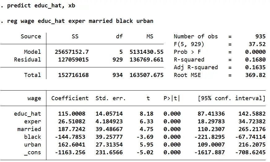
The second stage results thus allow us to make causal inference about a person’s education’s effect on their wages. In this regression, we can infer that for every additional year of education (‘educ_hat’), a person’s wages ‘wage’ goes up by $115. This parameter is also statistically significant at the 1% significance level since the p-value is less than 0.01.
2SLS Using the ivregress Command in Stata
To illustrate the workings of a 2SLS regression, we have seen a breakdown of how the two stages work. However, Stata also has a convenient command called ivregress that does a 2SLS regression for you in one go. The basic syntax for the ivregress command is as follows
ivregress 2sls depvar exo_varlist (endo_var = IV)
where depvar refers to our dependent variable, exo_varlist refers to all the exogenous independent variables in our structural equation, endo_var is our endogenous variable, and IV is the instrumental variable being used.
We also need to specify 2sls after the command name because it is one of the three estimators that this command deals with – the other two being LIML (Limited-Information Maximum Likelihood) and GMM (Generalised Method of Moments).
The command in our example above will look something like this. It should return the same parameters as the ones we obtained before in our second stage regression.
ivregress 2sls wage exper married black urban (educ=IQ)
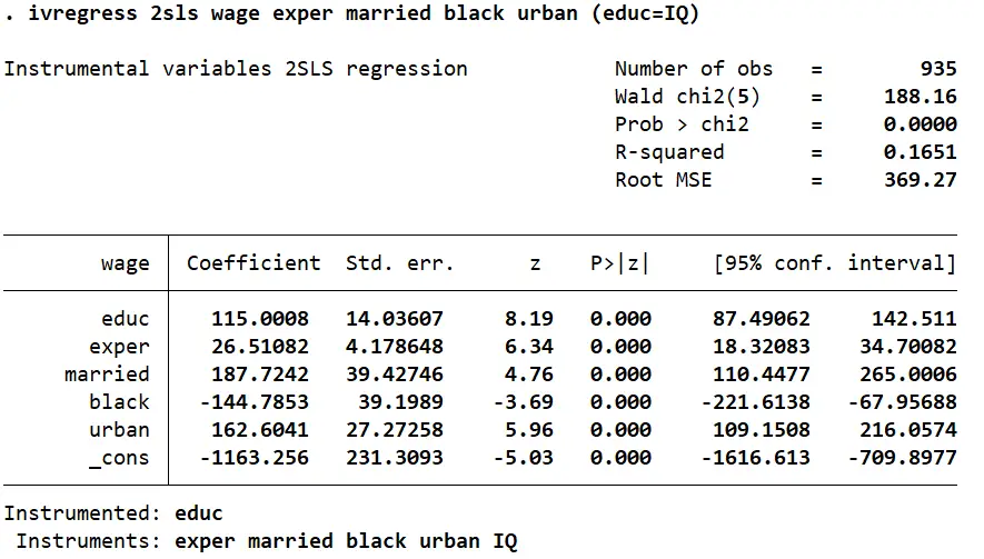
Note that while the parameters in a regression done using the ivregress command are the same as the second stage regression done manually, the standard errors from the ivregress results are lower than before. This is because when a 2SLS regression is done manually, Stata does not know that the ‘educ_hat’ values in the second stage are not real values but are in fact predicted values. It fails to make the relevant standard error adjustments.
ivregress takes this into account and produces consistent and valid standard errors which in turn ensure that our inferences are also valid.
In this case, while the difference between the two sets of standard errors is not too big and does not make lead to a change in our inferences, one should always use ivregress when doing a 2SLS regression in Stata to obtain valid and consistent results.
Testing for Endogeneity
We can test whether the 2SLS regression we ran was actually needed or not by testing if our regressors were endogenous or not. This can be done through a post-estimation command run after ivregress:
estat endog.
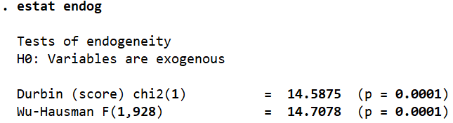
This command lets Stata run two tests with the null hypothesis that all of our variables were exogenous. We can use the p-values from these tests to accept or reject this hypothesis. In this case, both tests have a p-value of less than 0.01 which leads us to reject the null hypothesis and conclude that our structural equation did indeed suffer from endogeneity and a 2SLS regression was the right choice.
We can also test for endogeneity manually by obtaining the residuals from our first stage regression and using them as a regressor in our structural equation. The statistical significance of these residuals will indicate whether endogeneity exists or not.
reg educ IQ exper married black urban // first stage regression predict r, resid // predicting residuals from the first stage reg wage educ exper married black urban r // adding the residuals to our structural equation
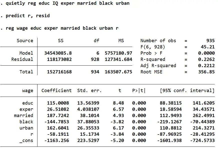
The coefficient for the residuals (‘r’) is statistically significant and indicates that endogeneity exists in the structural equation.
Reduced Form Regression
A regression type that you may encounter when looking into IVs is the reduced form equation.
A reduced-form equation is a regression of our dependent variable (‘wage’) on all the exogenous variables, including the IVs in our model.
A parameter for our endogenous variable can be obtained through a ratio of the reduced form coefficient for our IV, and the first stage coefficient for our IV.
A reduced form regression in our example can be run in Stata using the command:
reg wage IQ exper married black urban
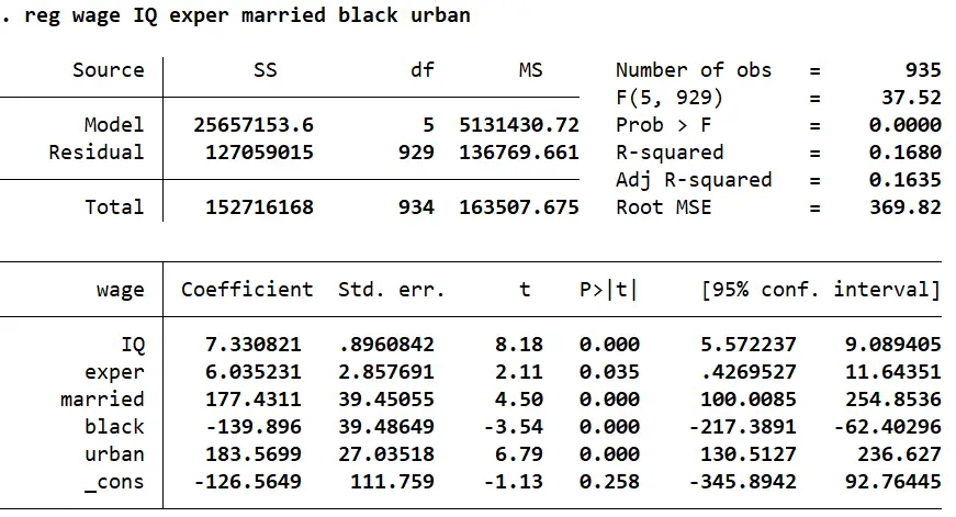
The coefficient for ‘IQ’ here is 7.330821.
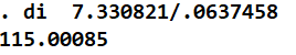
The coefficient for ‘IQ’ from our first-stage was 0.0637458.
Taking a ratio of the two returns us with the same parameter (115.00085) that we arrived at in our second stage regression or from the ivregress command:
di 7.330821/.0637458
Over-Identified, Just-Identified and Under-Identified Models
Depending on the number of IVs used in a model, we can classify regression models as over-identified, just-identified, or under identified depending.
An over-identified model has more instrumental variables (IVs) than the number of endogenous variables.
A just-identified model has an equal number of instrumental variables (IVs) and endogenous variables.
An under identified model has fewer instrumental variables (IVs) than the number of endogenous variables and thus cannot provide consistent and unbiased estimates of the endogenous variables’ coefficients.
In our example, we used one IV for one endogenous variable, making it a just-identified model.
IVs in Literature
Econometric literature offers an abundance of IV examples, some of which are very creative.
There are cases where endogeneity can arise from self-selection i.e. situations where a subject’s own bias and choices come into play when determining the independent variable (and by extension, the dependent variable). It is often difficult to identify or measure such biases quantitatively. Researchers then resort to instrumental variables (IVs) in their analysis to evade these biases and arrive at consistent and unbiased parameters.
Some very interesting and smart uses of IVs can be seen in papers like Angrist and Krueger (1991) who used a person’s quarter of birth (QOB) as an instrument to study the effect of the number of years of education on wages, and Angrist and Evans (1998) who use twin births as an IV to study the effect of family size on a mother’s labor supply.
Both these papers use IVs that are binary/dummy variables. Estimators where the instrumental variables are binary are called the Wald estimator, or the grouping estimator.