T-Test in R

In this article we will discuss t-test tactics in R thoroughly. T-test is a statistical tool used to compare the averages (mean) of two groups or samples and determines whether there is a statistically significant difference between them. T-test are especially helpful when working with small sample sizes (usually less than 30 observations per group). It takes into account the increased uncertainty that comes with smaller datasets, in contrast to other tests like the z-test that assume a normal distribution and are better suited for larger sample sizes.

Three different forms of t-tests are:

• One-Sample t-test in R
• Two Samples t-test in R
• Paired t-test in R

Each of which is designed for a certain set of data properties and research questions. Let’s understand it in R with a built-in dataset of cars.

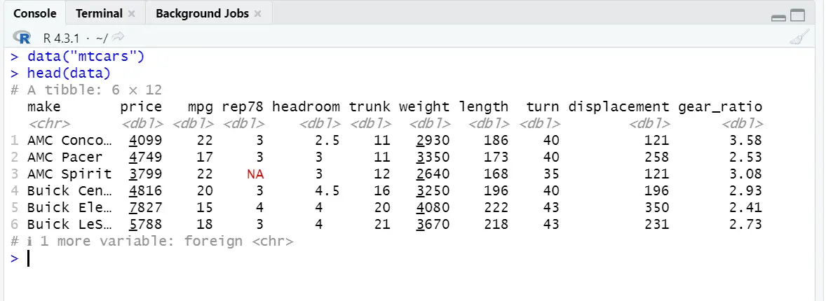
To analyze cars data, you can use R command to load it:

data("mtcars") head(data)

These commands will load the dataset and show the starting values of variables.

One-Sample t-test

One-sample t-test is used to detect whether a single sample’s mean substantially differs from a known or assumed population mean. It is frequently used in many study domains to draw conclusions about sample data in relation to a population parameter since it determines whether the sample mean is statistically different from the expected population mean.

Syntax for one sample t-test is:

 t.test(x, mu, alternative,..)

Here x is the numeric vector of sample for which we want to test mean, mu is the assumed mean for the population i.e. Null Hypothesis (H0), whereas, the Alternative Hypothesis (H1 or Ha) is any three values: “2-sided, greater, less”.

We will use “mtcars” dataset to get insights for one-sample t-test. Suppose that an analyst says average price of cars is $6,000. “Is there sufficient evidence to conclude that the average price of cars in the dataset is significantly different from $6,000?” For this question by default Two-tailed hypothesis (Non-Directional Hypothesis) will be:

H_o: Average price of car is $6000. (µ=$6000)

H_a: Average price of car is not $6000. (µ≠$6000)

R Code for one sample t-test for this question is

# Perform a one-sample t-test t_test_result <- t.test(data$price, mu = 6000)  # Print the t-test result print(t_test_result)

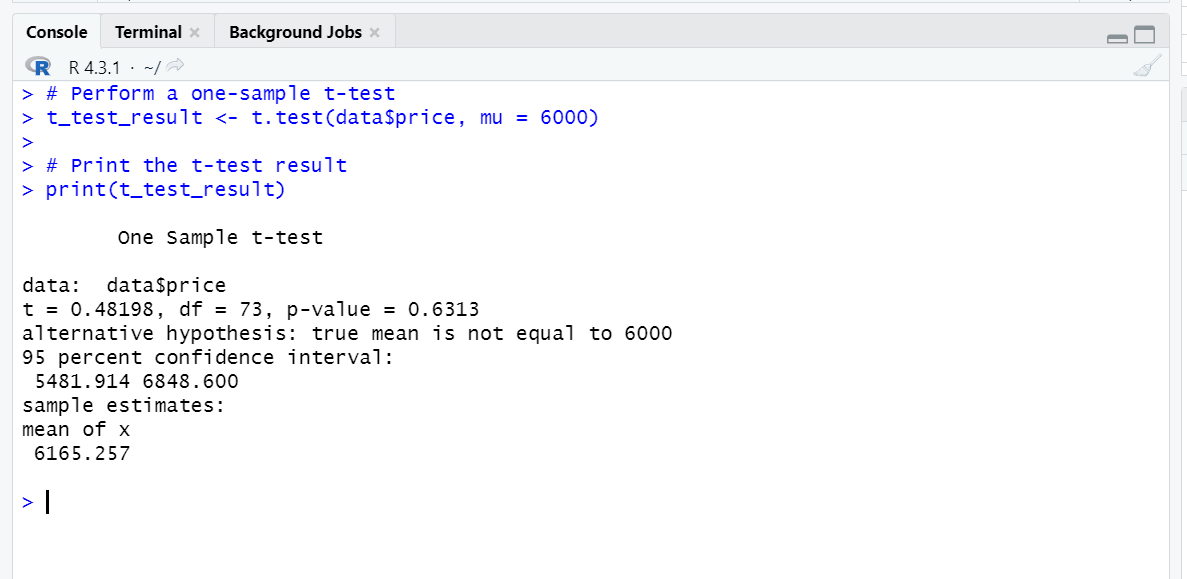
Lets understand the interpretation of t-test in R. t-value is 0.48198 and degrees of freedom is 73. p-value is 0.6313 which is above than our conventional significance level 0.05, hence we conclude that the null hypothesis is not rejected.

We do not have enough evidence to infer that the average price of cars in this dataset is higher or lower than $6,000 based on the outcomes and the p-value of 0.6313. This lack of a meaningful difference is further supported by the fact that the value of $6,000 is included in the 95% confidence interval.

Two-Sample t-test (Independent Sample t-test)

A two sample t-test is employed when comparing the means of two distinct groups or samples to see if they differ substantially from one another.

It is important to first understand the assumptions underlying this t-test and their implications. The two-sample t-test makes the assumption of homoscedasticity, often known as equal variances or homogeneity of variances. It implies that each group’s variance should roughly equal. Because it assumes that the variances are identical and pools the variances from both groups to estimate the common variance, this is also known as the “pooled variance t-test”. The validity of the test results may be impacted if this assumption is violated.

There are different methods to check and address the violation of two-sample t-test assumptions using statistical tests like Levene’s test. We may use the robust to unequal variances Welch’s t-test to determine whether variances are statistically different. Syntax for independent sample t-test is

 t.test(x, y , alternative = c("two.sided", "less", "greater"), mu = 0, paired = FALSE, var.equal = TRUE, conf.level = 0.95)

Here x and y are two variables for which we will check difference, alternative contains the directional or indirectional hypothesis, mu is population mean, paired is false here because we are doing independent samples test, var.equal is true because variances are assumed equal or pooled and conf.level is the confidence level.

For example if we want to know that “Do foreign and domestic cars in the ‘auto’ dataset have significantly different average prices?” we will use independent sample t-test.

R code for this is:

# Perform a two-sample t-test tst_test_result <- t.test(price ~ foreign, data =data)  # Print the t-test result print(tst_test_result ) 

Output:

The p-value, which is substantial at 0.6599, is significant. This implies that there is insufficient evidence to reject the null hypothesis and that there is no statistically significant difference between the true mean of “Domestic” and “Foreign” groups.

The average cost of cars in the “Domestic” category and the “Foreign” group are not significantly different, contrary to popular belief. Since zero is included in the 95% confidence range for the difference in means, the difference is not statistically significant.

We can perform it another way by splitting the column by category. 1 column for the prices of Foreign and one column for prices of Domestic Cars. R code for this process is

# Split the data into two groups based on the "foreign" variable foreign_group <- split(data$price, data$foreign)  # Perform a two-sample t-test t_test_result <- t.test(foreign_group$Foreign, foreign_group$Domestic)  # Print the t-test result print(t_test_result)

Output:

As we can see that results are same for both methods. There is no appreciable variation in the average car pricing between the “Foreign” and “Domestic” groups, supporting the previous view.

Paired Sample T-Test (Dependent Samples)

When comparing the means of two related or paired groups, such as before and after measurements on the same patient after a medication, a paired sample t-test is performed. The mean difference between paired observations is evaluated to see if it deviates significantly from zero.

The assumption of equal variances between the two sets of paired data is not as important in paired sample t-tests as it is in independent sample t-tests. This is due to the fact that the data’s paired nature tends to lessen the influence of variance differences. To understand this concept let’s take an example into account. We use chick weight built-in data from R. We want to check that “Does a specific treatment significantly impact the weight of chickens in the ‘ChickWeight’ dataset?

Syntax for paired sample

t-test is as t.test(x, y = NULL, alternative = c("two.sided", "less", "greater"), mu = 0, paired = TRUE, var.equal = FALSE, conf.level = 0.95)

Here x and y are two arguments for which we will perfom t-test, alternative contains the directional or non-directional hypothesis, mu is population mean, paired is true here because we are doing dependent samples test, var.equal is false so it will perform t-test assuming variance unequal and conf.level is the confidence level.

For paired-sample t-test we consider another dataset of chicks:

data("ChickWeight") head(ChickWeight)  # Filter the dataset to include only "Time" 0 and "Time" 2 paired_data <- ChickWeight[ChickWeight$Time %in% c(0, 2), ]  # Perform a paired sample t-test t_test_result <- t.test(paired_data$weight ~ paired_data$Time, paired = TRUE) # Print the t-test result  print(t_test_result)

A very low p-value of less than 2.2e-16 inferring that there is a significant difference in the mean weight of chicks between Time 0 and Time 2, this offers strong evidence to reject the null hypothesis. In conclusion, there is substantial evidence to show that there is a significant difference in the mean weights of chicks between Time 0 and Time 2, with weights decreasing by an average of 8.16 grams, based on the data and the extremely low p-value.