Standardization, normalization and mean centering of variable are common data processing techniques in Statistics and data analysis. It is important to standardize variables in statistics to compare and analyze different variables on the same scale. If you have two variables, one in inches and the other in centimeters, it’s not possible to compare these variables unless both variables are converted into one common comparable scale. Similarly, normalizing variables is important because it ensures that different features or variables in a dataset are on a similar scale. Imagine you have data on both people’s ages and their incomes. Because ages are typically small numbers and incomes can be large, the income variable might dominate the analysis simply due to its scale. Normalization scales all variables to a common range, often between 0 and 1, preventing one variable from overshadowing others.
Mean centering of variables is important because it helps remove the overall average or trend from the data, allowing you to focus on the variation or fluctuations around that average. In R, you can standardize, normalize and mean center the variable using various functions and packages.
Z-Score
One of the common and important way to normalize or standardize the variable is by using the z-score method. In this method, standardizing variables involves transforming the data so that it has a mean of 0 and a standard deviation of 1.
To use this method in R, let’s say we create a data set by using the following command
data <- c(10, 15, 8, 12, 18)
In mathematical terms, the scaled value of a variable is computed by subtracting the mean of the original variable from its raw value and then dividing the result by the standard deviation of the original variable. However, in R, all this can be done by using a simple function. To standardize the above data, we use the scale() function in R in a command, in the following way
standard<- scale(data)
The scale() function standardizes the data by default. You can access the standardized values using standard. The standardized data will have mean 0 and standard deviation of 1.

We can further check the mean and variance of data by using the following commands
mean(standard)
var(standard)
This was for the data set we create ourselves. However, when it comes to data sets having multiple variables of different kinds, we specify the variables we need to standardize. For instance, let’s say we want to use the mtcars data set. To load the data set, we use the following commands
data(mtcars)
Now, if we want to standardize the mpg variable, we first extract the variable and then standardize it using the scale() function. To extract and standardize the mpg variable, we use the following commands
mpg_variable <- mtcars$mpg
standard_mpg <- scale(mpg_variable)
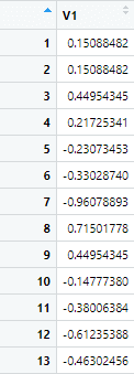
This will standardize the mpg variable, and the standardized variable will have the following data set.
This extracted variable, however, isn’t suitable to be used along with the rest of the data set. So if we want to standardize the variable, so that it stays along the rest of the data set, we can use the following command.
mtcars$st_mpg <- scale(mtcars$mpg)
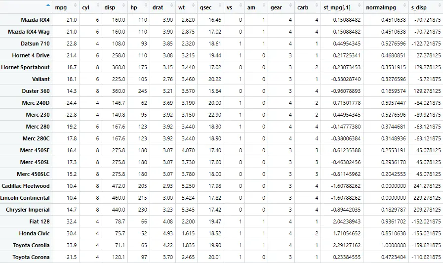
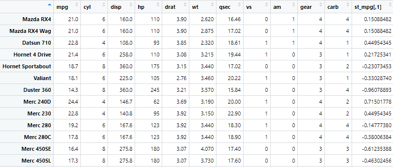
This command creates another variable st_mpg which is short for standardized mpg, which has the standardized values for the mpg variable. The data with standardized variable will look like following
Normalize a Variable in R
Normalization scales the data to a specific range, often between 0 and 1. You can normalize a variable in the mtcars dataset, let’s say the mpg variable, to the [0, 1] range, by using the following command This method is also called min max normalization.
mtcars$normalmpg <- (mpg_variable - min(mpg_variable)) / (max(mpg_variable) - min(mpg_variable))
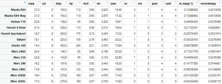
In this example, the “normalmpg” variable is calculated by subtracting the minimum value of the original mpg variable and then dividing by the range (the difference between the maximum and minimum values). This ensures that the normalized values fall within the [0, 1] range. This produces the following results
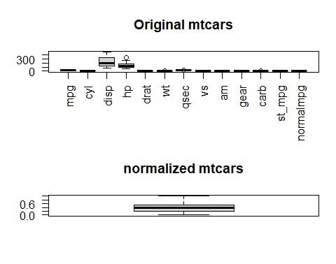
If we want to visualize mpg variable before and after normalization, we can do that by creating box plots for the variable using following command
par(mfrow = c(2, 1)) boxplot(mtcars, main = "original mtcars", las = 2) boxplot(mtcars$normalmpg, main = "normalized mtcars", las = 2)
In the above command, we first set up a 2×1 grid for side-by-side plots. Then create the first boxplot for the original mtcars dataset using boxplot() function and then create the second boxplot for the standardized mpg variable.
The boxplots created from the above commands are following
Mean Centering in R
Mean centering is a data preprocessing technique that involves subtracting the mean of a variable from each individual data point in that variable. This process results in a new variable where the mean is shifted to zero, and each data point represents the deviation from the original mean.
To do mean centering of a variable, say displacement, we use the following command
mtcars$s_disp <- mtcars$disp - mean(mtcars$disp, na.rm = TRUE)
In the above command, we perform mean centering by subtracting the mean from each value in the “disp” variable. The mean() function is used to calculate the mean (average) of the variable disp_variable. The na.rm = TRUE argument is included to handle missing values (NA) in the variable. The following variable named “s_disp” is mean centered.