In the previous article, we discussed the theoretical aspects of the estimation strategy. In this article will look into the practical aspects of the estimation strategy (Between estimation, First difference estimation, and within estimation).
Between Estimation:
We will first implement the manual method of between estimation analysis and then use the Stata command to do between estimation analysis. Before starting the analysis, we will keep only the variable we are interested in by using the below command:
Download Example Filekeep idcode year ln_wage hours
Firstly, we will calculate the averages of ln_wage and hour using the below command:
collapse (mean) ln_wage hours, by(idcode)
The collapse command calculates the mean and the variables for which we want to calculate the mean, such as ln_wage and hours. Finally, after the comma, we use the by function to tell Stata the variable based on which we want to take the averages. In this command, we take the average for each idcode.
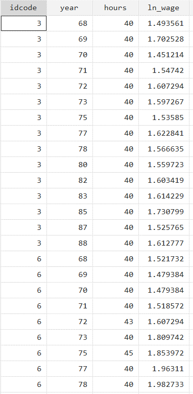
The data before the collapse look like this:
After running the above command, the data will look like this:
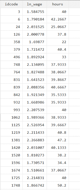
Each idcode will now have a single value. Next, we will run the Pooled OLS using the below command:
regress ln_wage hours
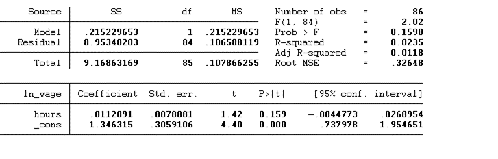
The above figure represents the results of the Pooled OLS regression. The p-value> 0.05, which indicates that there is no significant effect of hours on the ln_wages.
Now we will use the Stata command to perform between estimate analysis. Firstly we will tell stata that our data is a panel by using the below command:
xtset idcode year
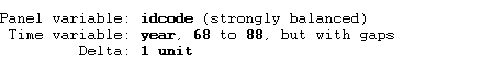
The data is strongly balanced. Balanced panel data refers to a dataset where all entities, or observation units, are observed for an equal and consistent number of time periods. Now we will reg the independent variable against the dependent variable using between estimation command given below:
xtreg ln_wage hours, be
xtreg is the command, ln_wage is the dependent variable, and hours are the independent variables. The be after the comma is the function that represents the model we want to use.
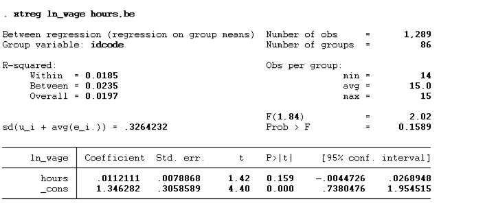
You will notice that manual and Stata commands for between estimation will provide the same results.
First Difference Estimation:
We will use the national longitudinal survey of young women’s dataset for the first difference estimation. The data is the panel. The dataset can be accessed by using the below syntax:
webuse nlswork, clear
The data comprises of 28000 observations approximately. However, we will only keep the data of years 68 and 69 for this analysis. To do so, we will use the below command:
keep if inlist(year,68,69)
keep command tells Stata you want to keep certain observations in the dataset. if used to specify a condition that the observations must meet to be kept. inlist function checks if a variable’s value is in a specified list of values. Inside the parentheses, you specify the variable year and the values 68 and 69. So the condition being checked is whether the year’s value is 68 or 69.
Then we will run a command to tell Stata that our data is panel by using the below command:
xtset idcode year
Next, we will use the below command to reg the first difference of independent variables against the first difference of dependent variables. The command is given below:
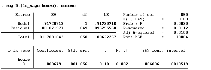
reg D.(ln_wage hours), nocons
reg command tells Stata you want to perform a linear regression. D. indicates that you want to use the first differences of the variables within the parentheses. This means the model will be estimated based on the change in ln_wage and hours from one period to the next rather than their levels. So, the dependent variable in this regression is the first difference of ln_wage, and the independent variable is the first difference of hours. nocons option tells Stata not to include an intercept (constant term) in the regression model.
We are now performing the first difference manually to get a clearer understanding. First, we will calculate the first difference of both dependent and independent variables using the below command:
gen diff_ln_wage=D.ln_wage gen diff_hours=D.hours
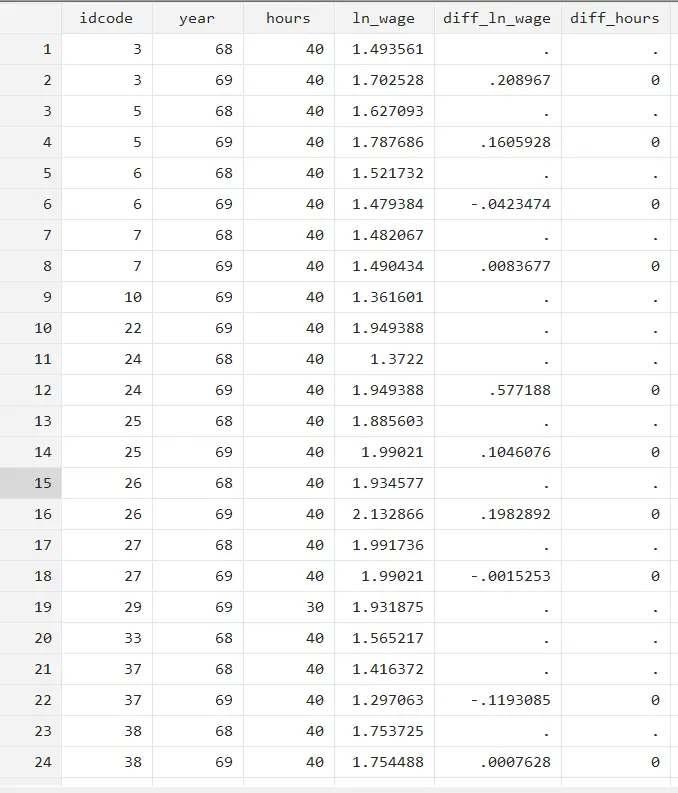
Two new variables will be generated, representing the differences in ln_wage and hours. Then we will run the regression using the newly generated variables:
regress diff_ln_wage diff_hours,nocons
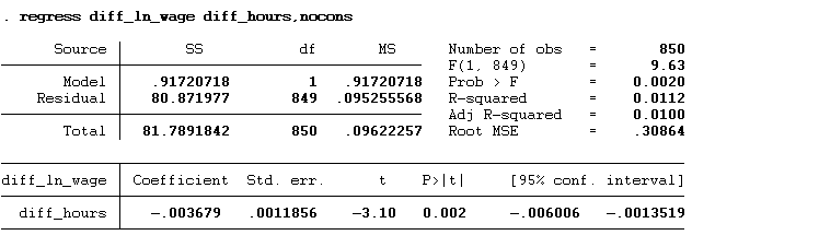
The p-value < 0.05, which means that the first difference of hour has a significant influence on the first difference of ln_wage. The impact of hours is negative on the ln_wage.
Within Estimation:
To perform within estimation, first, we will generate mean using the below commands:
bys idcode: egen mean_ln_wage=mean(ln_wage) bys idcode: egen mean_hours=mean(hours)
The bys tells Stata that you want to perform the subsequent command separately for each unique value of the variable idcode. Stata will sort the data by idcode and then perform the following command within each group of identical idcode values. This part of both commands uses the egen function to create new variables, mean_ln_wage, and mean_hours, that store the mean of the variable ln_wage and hour within each group of idcode. Every observation with the same idcode will have the same value for mean_ln_wage and mean_hours, equal to the mean of ln_wage and hours for that idcode. Next, we will calculate the demean of each value using the below command:
gen demeaned_ln_wage=ln_wage-mean_ln_wage gen demeaned_hours=hours-mean_hours
The gen command tells Stata to generate a new variable, and the expression on the right side of the equal sign calculates the value of that variable for each observation. Specifically, for each observation, it subtracts the mean_ln_wage and mean_hours from the value of ln_wage and hours. Assuming that mean_ln_wage and mean_hours contain the mean of ln_wage and hours for each group identified by some other variable (e.g., idcode), as in the commands you provided earlier, this subtraction will demean ln_wage and hours, removing the group-level mean. Lastly, we will run the regression using the below command:
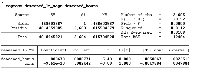
regress demeaned_ln_wage demeaned_hours
We will get the below results on running the above command: