
In the previous 3 articles, we discussed the theoretical and practical implications of the Pooled OLS, Fixed Effect, and Random Effects Models and the significance of dummy variables such as time or industry dummies. This article will look into other techniques that come under panel data analysis. The techniques are listed below:
Download Example File- Between Estimate (BE)
- Within-group Estimate (WG)
- First Difference Estimate (FD)
In our previous three articles, we discussed the problem of heterogeneity and how we can use the least squared dummy variable (LSDV) to resolve this problem. Two more models can be used to deal with the heterogeneity problem, including the within-group estimate and the first difference estimate.
Between Estimation:
Between estimation focuses on variations between entities and effectively ignores the time dimension of the data. The step included in the between estimation are:
- Take an average of dependent and independent variables.
- Run OLS regression on the averages.
When we take averages and collapse the data, it no longer retains the panel structure. Instead, it becomes cross-sectional data.

In the above equation, “it” represents that data is the panel. In between estimations, we take the average. For example, if we have three firms with ten-year data, we will take the average of these 10 years. We will be left with a single value for each firm. So, after collapse (taking averages), the equation will look like this:
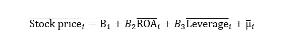
Only “i” is left, and “t” has been removed. This shows that the time dimension has collapsed. Once getting this average, we will run OLS regression on it.
The limitation of this method is that we lose the richness of the panel data. We collected the panel data and then converted it into cross-sectional data. That’s why this method is rarely used.
The Problem of Heterogeneity and Endogeneity:
In the first article, we discussed the issue of heterogeneity and endogeneity in the case of the Pooled OLS model. Let’s recall it again. Some unobserved factors also impact the dependent variable (stock price), such as two-time invariant factors, firm culture, and organizational culture. As we can’t observe these factors, we call them individual heterogeneity, unobserved heterogeneity, and unobserved firm-specific characters that would impact the stock price. These factors affect go into the error term.
Suppose the organizational culture (time-invariant variable) is an unobserved factor that affects the stock price.

Let’s donate this OC as “αi”. Here, “i” shows that this variable is time invariant as it does not change with time.
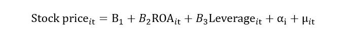
All the time-invariant unobserved factor effect will go into the “αi”. Both αi and μit will form the composite error term “νit”. This composite error term includes the impact of individual heterogeneity and random error. Now, if this νit correlates with the ROA, then it leads to the problem of endogeneity. Hence, it is a must to deal with it.
First Difference Estimation:
First difference estimation is a method used in panel data analysis to control time-invariant unobserved effects. By looking at the change in the variables from one period to the next it helps to eliminate potential bias from factors that don’t change over time but aren’t directly included in the model.
The steps include the following:
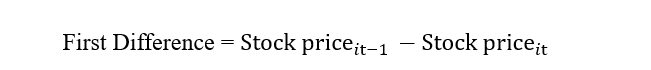
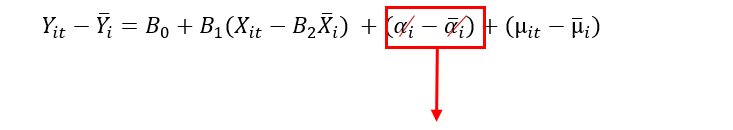
- Take the first difference between dependent and independent variables. The first difference is between a variable’s lag and current value. The formula is:
2. Then we will run the OLS on the first difference.
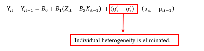
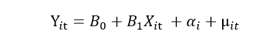
Suppose we have an equation:

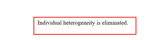
Here Yit is the dependent variable, βo is the intercept, β1Xit is the independent variable, αi is the unobserved time-invariant factor, and μit is the random error term. We take the difference of each variable. So, when we take the difference, the lag value will be subtracted from the current value. For example, the αi at number 5 will be subtracted from the αi at number 5. Hence the two values cancel each other, and we successfully eliminated the heterogeneity error from the model.
The limitation of using the first difference variable is that we can’t include time-invariant variables, such as gender or race. Another limitation is that we lose many observations.
Within Estimation:
Within estimation focuses on analyzing the variations within each individual or entity over time, thus eliminating the influence of time-invariant unobserved heterogeneity.
Within estimation is done in three steps that include:
- Take an average of dependent and independent variables.
- Deduct these averages from the relevant variables.
- Run OLS regression on time-demeaned variables.
hat we will do is we will take an average of each variable and then deduct this average from each observation of the variable as shown below equation:
We know that the average of the constant is constant. So, by doing this, we will eliminate individual heterogeneity.
The limitation of the within estimation is that we can’t include time-invariant variables, such as gender or race. We will get the same result from all these methods.