
In R Programming, logistic regression is a grouping approach used to determine the likelihood of happening success and failure. When the dependent variable is binary (0/1, True/False, Yes/No), logistic regression is implemented. In a binomial distribution, the logit function is leveraged as a link function.
The logistic function, frequently known as the sigmoid function, is the core notion that subsequent logistic regression. In logistic regression, this sigmoid function is used to reflect the relationship between the predictor variables and the likelihood of the binary result.
Logistic regression is a statistical procedure for dealing with binary categorization problems. To fit logistic regression models in R, use the glm function. Here’s a simple example.
# Install and load packages install.packages("caret") library(caret) # caret is useful in switching between models/ partitions # Set seed for reproducibility set.seed(123) # Generate sample data data <- data.frame( heart_attack = sample(c('Yes', 'No'), 500, replace = TRUE), exercise = sample(c('Yes', 'No'), 500, replace = TRUE), bmi = sample(20:50, 500, replace = TRUE), gender = sample(c('Male', 'Female'), 500, replace = TRUE) ) # Convert 'Yes'/'No' to 1 or 0 for the 'heart_attack' variable data$heart_attack <- ifelse(data$heart_attack == 'Yes', 1, 0) # Split the data into training and testing sets index <- createDataPartition(data$heart_attack, p = 0.8, list = FALSE) train_data <- data[index, ] test_data <- data[-index, ] # Fit logistic regression model on the training data model <- glm(heart_attack ~ exercise + bmi + gender, data = train_data, family = "binomial") summary(model) # Make predictions on the testing data predictions <- predict(model, newdata = test_data, type = "response") # Convert probabilities to binary predictions (0 or 1) binary_predictions <- ifelse(predictions > 0.5, 1, 0) # Evaluate the accuracy of predictions accuracy <- sum(binary_predictions == test_data$heart_attack) / nrow(test_data) cat("Accuracy on the testing data:", accuracy, "\n")Let’s understand the dataset code for clarification.
“Set.seed(123)” Sets the seed for the random number source. This affirms that if one runs the code again, he’ll receive the same random numbers, entitling him to regenerate the results. “data.frame(…)” evokes a data frame named data with four columns (heart_attack, exercise, body mass index, and gender). “sample(c(‘Yes’, ‘No’), 500, replace = TRUE)” creates a random sample of 500 elements from the vector ‘Yes’ and ‘No’ with replacement. This is used to induce values for the variables heart_attack and exercise. Similarly “sample(c(‘Male’, ‘Female’), 500, replace = TRUE)” generates a random sample of 500 male and female gender variable values. “ifelse” function, converts the ‘Yes’/’No’ values in the heart_attack column to 1 and 0, respectively. This is executed to transform the response variable into a binary layout that may be used in logistic regression. The glm function’s (family = “binomial”) stipulates that logistic regression should be used. “Fit” fits a logistic regression model using the glm function. Heart_attack is the response variable, and exercise, bmi, and gender are predictor variables. Logistic regression is indicated by the family = “binomial” argument.
Using the “createDataPartition” function from library caret, this code first detaches the data into training and testing groups. The model is then fitted to the training data and predictions are made on the testing data. Finally, it evaluates the predictive reliability on the testing data.
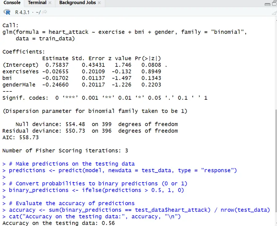
Each coefficient’s p-value (Pr(>|z|)) reveals whether the variable is statistically significant in foreseeing the response variable. At the 0.05 significance level, the lingering factors do not manifest to be statistically significant. The log-odds of having a heart attack lessen by 0.01702 units for every unit increase in BMI (Body Mass Index), providing all other variables in the model do not fluctuate.
In simplistic terms, people with a higher BMI have a little bit lower risk of having a heart attack, based on this model. However, when estimating coefficients, statistical significance should be assessed, and the p-value for “bmi” is 0.1343, which is higher than the conventional significance level of 0.05. As a result, in this scenario, the effect of BMI on the risks of having a heart attack is statistically insignificant.
The goodness-of-fit test engages null deviance and residual deviance. The AIC (Akaike Information Criterion) is a model goodness of fit standard that imposes the penalty for the number of parameters. In general, lower AIC values indicate a better-fitting model.
Accuracy on testing data shows that predictions are 56% accurate. This signifies that for 56% of the occurrences in the testing dataset, the model precisely predicted the outcome (heart attack or no heart attack). Remember that accuracy is only one measure. Depending on the context of this situation, one may want to examine other evaluation metrics.
Memorize that the meaning of logistic regression coefficients is in terms of log-odds, and one may want to revise these to odds ratios for a more natural reading if necessary.