
Normality refers to the typical feature of a normal distribution, which is a precise type of probability distribution with uncommon qualities that make it particularly relevant for various statistical investigations.
In many statistical analysis, determining whether your data follows a normal distribution requires checking the normality of data. There are different ways to check for normality in R. For understanding we will use built-in dataset “iris”. It contains measurements of 150 iris flowers. To load dataset the function is:
# Load the Iris dataset data(iris) # View the first few rows of the dataset head(iris)
Histogram:
To prominently evaluate the distribution of your data, you can generate a histogram. Create a histogram with the ‘hist()’ function and look for a bell-shaped curve. Here’s the code:
# Generate a histogram # Create a histogram for Sepal.Width hist(iris$Sepal.Width, main="Histogram of Sepal.Width")
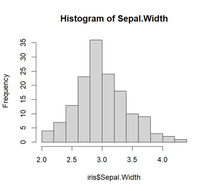
As is seen from the histogram graph is bell shaped, can be said to be symmetrical. We can say that variable sepal width is normally distributed.
Now for the variable sepal length function is:
# Generate a histogram # Create a histogram for Sepal.Length hist(iris$Sepal.Length, main="Histogram of Sepal.Length")
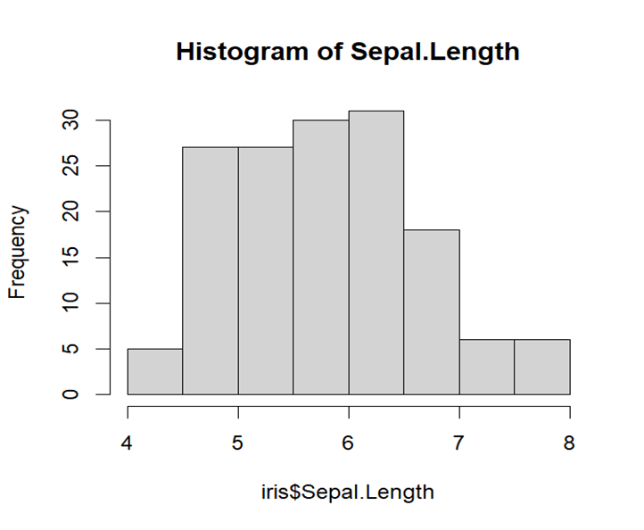
This graph does not show any pattern like bell shaped or symmetry which means its distribution is not normal. Data has variability in itself and more peaked which means it is not symmetrical to its mean, median or mode.
Density Plot
Now for density plot, the function that is used to access normality by density plot is:
For Sepal Width
# Create a density plot for Sepal.Width plot(density(iris$Sepal.Width), main="Density Plot of Sepal.Width")
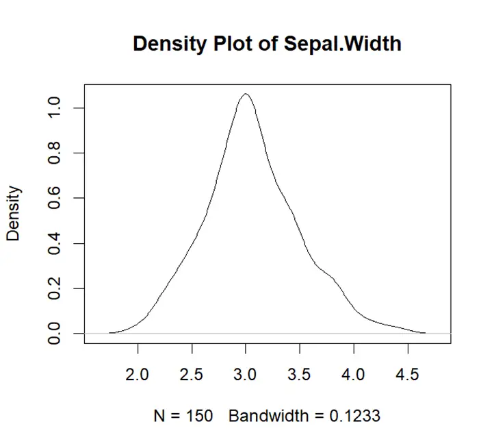
This density plot is symmetric showing that the data is symmetrical around its central tendency. There is only one peak in the density plot which shows data is unimodal. Right side of plot is wider than left which means there is more variability.
For Sepal Length:
# Create a density plot for Sepal.Length plot(density(iris$Sepal.Length), main="Density Plot of Sepal.Length")
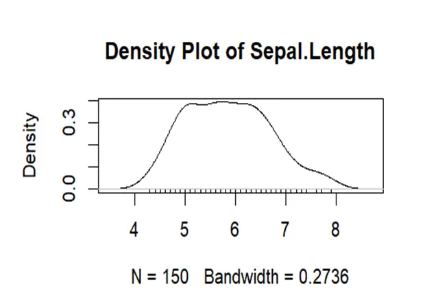
It can be seen from the density curve that it has heavier tails than sepal width as well as more spread. It has more than 1 peaks which shows it is not unimodal. So it departs from normality.
Normal Q-Q Plot:
A quantile-quantile (Q-Q) plot compares your data’s quantiles to the quantiles of a theoretical normal distribution. If your data has a normal distribution, the Q-Q plot points should closely follow a straight line. The ‘qqnorm()’ and ‘qqline()’ functions can be used to generate a Q-Q plot:
For Sepal Width:
# Create a Q-Q plot for Sepal.Width qqnorm(iris$Sepal.Width) qqline(iris$Sepal.Width)
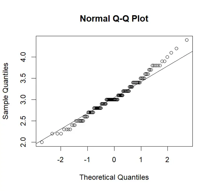
In Q-Q plot a straight line can be seen. Straight line shows normality but some points are above the line which shows heavier tails. Heavier tails mean data has more variability. We can say that data of sepal width approximately follows normal distribution.
Now look for the Q-Q plot of the variable sepal length.
# Create a Q-Q plot for Sepal.Length qqnorm(iris$Sepal.Length) qqline(iris$Sepal.Length)
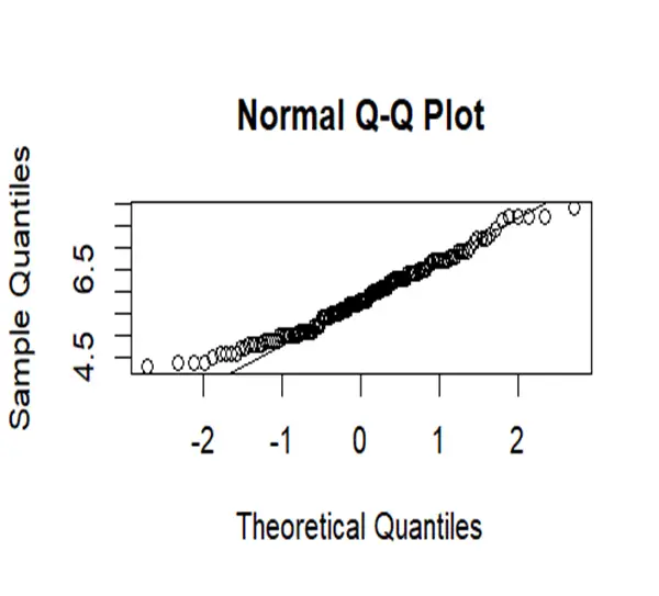
Data of sepal length has more variability as points are scattered from line at ends.it has heavier tails and skewed at right side. So it is fully departs from normality.
Shapiro-Wilk Test:
The Shapiro-Wilk test is a proper statistical test that is used to conclude normality. You can use the function shapiro.test()
The null hypothesis of this test is that data is normally distributed. One cannot reject the null hypothesis that the data follows a normal distribution if the p-value is greater than selected significance threshold (e.g., 0.05).Lets understand it with examples:
# Perform the Shapiro-Wilk test for Sepal.Width shapiro.test(iris$Sepal.Width)
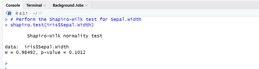
The p-value of Shapiro-Wilk test is 0.1012, which is above the standard significance level of 0.05. It indicates that we have less enough evidence to reject the null hypothesis of normality in data.
Now for sepal Length
# Perform the Shapiro-Wilk test for Sepal.Length shapiro.test(iris$Sepal.Length)
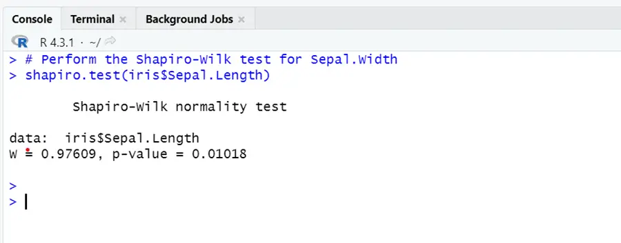
Sepal length variables vary significantly from normal distribution. Low p- value tends us to reject the null hypothesis of normality.
Skewness-Kurtosis Test
Skewness is a measure that is used to evaluate symmetry in the distribution of data whereas kurtosis evaluates degree of tail and peak in distribution of data.
To check kurtosis and skewness in R we will use functions:
# Extract the "Sepal.Length" variable sepal_length <- iris$Sepal.Length skew <- skewness(sepal_length) kurt <- kurtosis(sepal_length) # Display the results cat("Skewness: ", skew, "\n") cat("Kurtosis: ", kurt, "\n\n")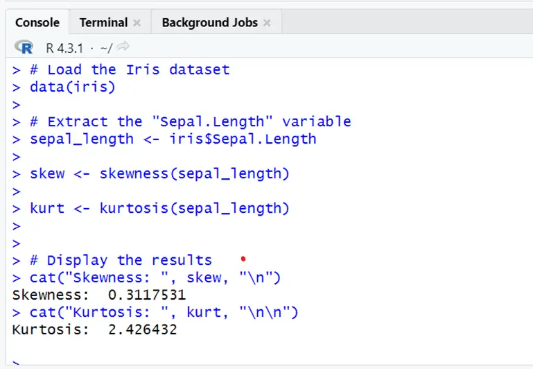
Sepal length is positively skewed to the right slightly and have a longer tail. Kurtosis value shows the heavy tailedness and more peak than the normal distribution. So it deviates from normal distribution.
If we do the same for sepal width the function is:
# Extract the "Sepal.Length" variable sepal_width <- iris$Sepal.Width skew <- skewness(sepal_width) kurt <- kurtosis(sepal_width) # Display the results cat("Skewness: ", skew, "\n") cat("Kurtosis: ", kurt, "\n\n")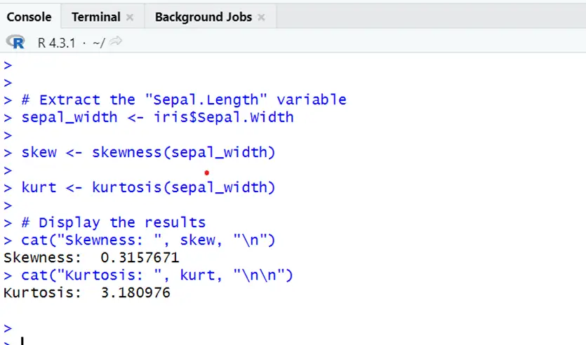
Sepal width also showing positive skewness slightly to the right side and kurtosis showing heavy tail deviating from normal as it will normal if kurtosis=3 and skewness 0.
On the basis of results of these two variables we can access that variable sepal length is perfectly deviates from normality but in case of variable sepal width we can say that it is approximately normal as its extent of variation not too large.
If it is necessary to meet the assumption of normality one must move to the non-parametric approaches.